Long short-term memory or LSTM are recurrent neural nets, introduced in 1997 by Sepp Hochreiter and Jürgen Schmidhuber as a solution for the vanishing gradient problem.
Recurrent neural nets are an important class of neural networks, used in many applications that we use every day. They are the basis for machine language translation and perform speech recognition when we interact with digital assistants on our devices.
Recurrent neural nets
The key feature of recurrent neural nets (RNN) is that they work well with sequence data. These can be sentences, which are just sequences of words, series of prices of financial securities or some other form of sequence. Another distinction of RNNs is that they remember what they learnt from previous inputs fed to the RNN when generating predictions for the current input.
This distinguishes them from normal feed forward networks which produce the output based on the current input only. When predicting whether a current image is a cat or dog, we do not directly consider what was the classification on the previous image that we examined with the neural net.
Information about the prior input and outputs of recurrent neural nets are contained in the so-called hidden states of the recurrent neural network. In figure 1 which shows the architecture of the recurrent neural net, hidden states are denoted as h(t-1), h(t) and h(t+1):
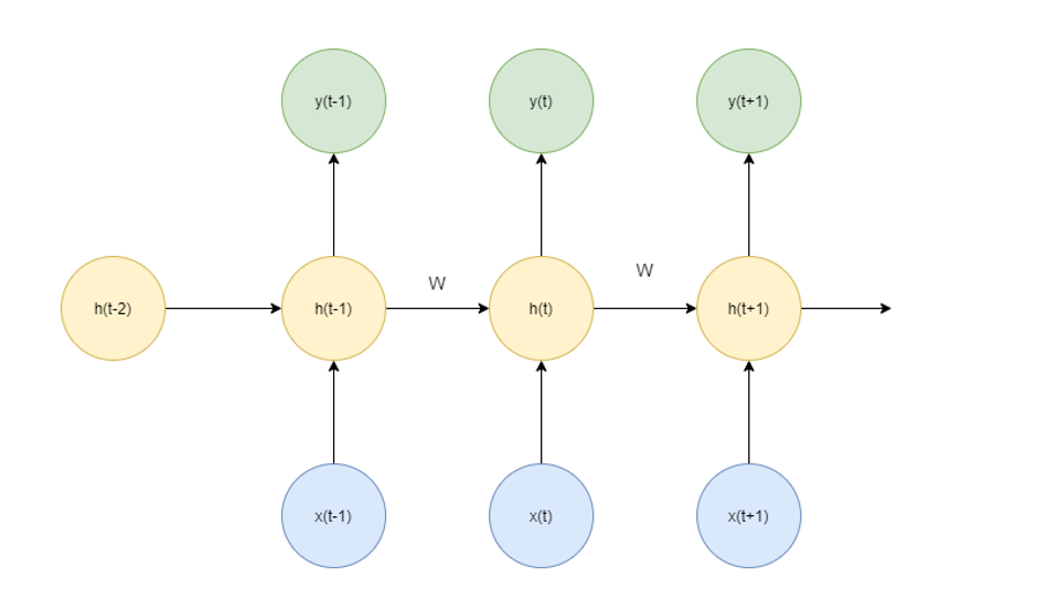
Figure 1: Recurrent neural net
Types of recurrent neural nets
There are several types of recurrent neural nets (RNN) available, including:
- Encoder decoder or sequence to sequence RNNs,
- Bidirectional RNNs,
- Recursive RNNs,
- Gated Recurrent Unit (GRU),
- LSTM RNNs.
Encoder decoder RNNs
Encoder decoder RNNs consist from two main parts: encoder and decoder. Encoder encodes the input, which can be a sentence in source language (translation task) or a question (question & answering task). Encoder produces the final hidden state or encoder vector, which captures the information contained in all inputs. This is then sent to the decoder, which produces the output sequence, which can be a translated sentence or an answer to the question.
One of the strengths of the encoder decoder RNN architecture is that the lengths of the input sequence and output sequence do not necessarily have to be the same.
Bidirectional RNNs
Bidirectional RNNs modify the RNNs in that the inputs are processed both on forward and backward basis. Consider the following sentence:
This is a __(target prediction)__ book about John Rockefeller.
Bi-directional RNN that considers the context which comes after the target would be more accurate in prediction than the normal RNN. Bi-directional RNNs use two RNNs, one for forward direction processing and one for backward direction. The hidden states from both RNNs are then concatenated in a single hidden state.
Bi-directional RNNs can be slow as they must perform both forward and backward passes. They are typically used for specific applications, e.g. named entity recognition.
Limitations of standard RNNs – Vanishing Gradient Problem
Standard method of training RNNs is backpropagation through time or BPTT, which generalize the backpropagation algorithm for feed forward neural networks.
When training neural nets (NN) with backpropagation, the updates to the NN’s weights are proportional to the partial derivatives of the loss function with respect to weights on each iteration step. In certain cases, gradients can become vanishingly which may prevent the neural net to further improve during training. LSTM solves this vanishing gradient problem with memory cells which lead to continuous gradient flow and with errors preserving their values.
LSTM
Let us now try to better understand the structure and the working of LSTM neural nets.
The key concept of the LSTM is cell state or the “memory state” of the network, which captures information from previous steps. Information is added to the cell state with several different gates: forget gate, input gate and output gate. Gates can be thought of as control units that control which data is added to the cell state.
The first important gate of the LSTM is the forget gate. Forget gate processes the previous hidden state and the current input by applying the sigmoid function, which maps the final value to the interval between 0 (forget data) and 1 (pass it through unchanged).
Next, we pass the previous hidden state and the input to the sigmoid of the input gate and also pass hidden state and current input to the tanh function, followed by multiplying both sigmoid and tanh output.
All these values are then used to update the cell state, by first multiplying cell state by vector from the forget gate. This is then pointwise added to the vector from the input gate, to obtain the new, updated value of the cell state.
LSTM is then concluded with the final, output gate. Its output is computed by first passing previous hidden state and the input to the sigmoid function and then multiplying this with the updated state that was passed to the tanh function. The output is the new hidden state which is passed to the next time step along with the new cell state.
We will now implement a LSTM deep neural network and use it to predict sentiment of movie reviews from the IMDB data set.
LSTM with python
First step is to load the required libraries and models:
import pandas as pd

import numpy as np

import sklearn

from sklearn.model_selection import train_test_split

from sklearn.metrics import classification_report,roc_auc_score,confusion_matrix,accuracy_score,f1_score,roc_curve

from sklearn.preprocessing import LabelEncoder

from keras.preprocessing.sequence import pad_sequences

from keras.models import Sequential

from keras.callbacks import ReduceLROnPlateau, EarlyStopping

from keras.layers import Activation, Dense, Dropout, Embedding, LSTM

import re

from IPython.display import display

import os

import string

import time

import random

import matplotlib.pyplot as plt

from tensorflow.keras.datasets import imdb

random.seed(10)
Importing data
We will use the movie reviews data set, containing 25,000 movies reviews from IMDB, that were labelled by sentiment as positive or negative.
Reviews have already been pre-processed, with each review encoded as a sequence of word indexes (integers). For convenience, words are indexed by their overall frequency in the dataset, so that for instance the integer “10” encodes the 10th most frequent word in the data.
This enables filtering operations, e.g. we can consider only the top 5000 most common words. As a convention, “0” does not stand for a specific word, but instead is used to encode any unknown word.
keras function load_data returns 2 tuples:
- x_train, x_test: list of sequences, which are lists of indexes (integers),
- y_train, y_test: list of integer labels (1 or 0).
Preparing the train and test data sets:
num_words = 5000

( X_train , y_train ),( X_test , y_test ) = imdb.load_data(num_words = 5000)
As reviews have different number of words, the lists or sequences in X_train do not have the same length. To ensure that, we pad 0s in the beginning of each sequence, with maxlen parameter specifying the target length of sequences:
sequence_length = 300

batch_size = 128

X_train_seq = pad_sequences( X_train, maxlen = sequence_length)

X_test_seq = pad_sequences( X_test, maxlen = sequence_length)
We will also use LabelEncoder for target variable:
encoder = LabelEncoder()

encoder.fit(y_train)

y_train_transformed = encoder.transform(y_train).reshape(-1,1)

y_test_transformed = encoder.transform(y_test).reshape(-1,1)
We will use word embedding approach to represent words with numerical vectors. Vectors of words are learned as part of the training procedure and following the principle that the meaning of the word can be inferred by the words that surround it. Word embedding vectors of semantically similar words are thus more closely aligned in word vector space than those of semantically dissimilar words.
Keras provides an Embedding layer for this purpose. It only accepts integer indexes for words, which means that one needs to carry out tokenization as part of pre-processing, e.g. using Keras own Tokenizer for this purpose.
In our case, this was already done with our reviews already in the form of integer indices, so we do not need the Tokenizer and its application.
Keras Embedding layer can be used in a variety of ways. We can use it to train a word embedding and then use it in another model. We can train the word embedding as part of the deep neural net training. Or we can load a pre-trained word embedding model to the Keras embedding layer.
In our case, we will select the second option and learn the embedding of words along with the rest of the deep neural net.
Each Keras embedding layer requires three parameters:
- input_dim or size of the vocabulary,
- output_dim or dimension of the word embedding space,
- input_length or the length of input sequences.
e = Embedding( num_words , 10 , input_length = sequence_length )
Our input data consists of sequences of words or their indices after transformation.
Long short-term memory (LSTM)
Our neural net consists of an embedding layer, LSTM layer with 128 memory units and a Dense output layer with one neuron and a sigmoid activation function.
We next train the LSTM model for 5 epochs and evaluate it on the test set:
model = Sequential()

model.add(e)

model.add(LSTM( 128 , dropout = 0.25, recurrent_dropout = 0.25))

model.add(Dense(1, activation = 'sigmoid' ))

model.summary()

model.compile( optimizer = "adam" , loss = 'binary_crossentropy' , metrics = ['accuracy'] )

early_stopper = EarlyStopping( monitor = 'val_acc' , min_delta = 0.0005, patience = 3 )

reduce_lr = ReduceLROnPlateau( monitor = 'val_loss' , patience = 2 , cooldown = 0)

callbacks = [ reduce_lr , early_stopper]

train_history = model.fit( X_train_seq , y_train_transformed , batch_size = batch_size, epochs = 5,validation_split = 0.1 , verbose = 1 , callbacks = callbacks)

score = model.evaluate( X_test_seq , y_test_transformed , batch_size = batch_size)

print( "Accuracy: {:0.4}".format( score[1] ))

print( "Loss:", score[0] )
Layer (type) Output Shape Param #
=================================================================
embedding_1 (Embedding) (None, 300, 10) 50000
_________________________________________________________________
lstm_1 (LSTM) (None, 128) 71168
_________________________________________________________________
dense_1 (Dense) (None, 1) 129
=================================================================
Total params: 121,297
Trainable params: 121,297
Non-trainable params: 0
_________________________________________________________________
Train on 22500 samples, validate on 2500 samples
Epoch 1/5
22500/22500 [==============================] – 661s 29ms/step – loss: 0.5861 – acc: 0.6949 – val_loss: 0.4112 – val_acc: 0.8176
Epoch 2/5
22500/22500 [==============================] – 627s 28ms/step – loss: 0.4313 – acc: 0.8091 – val_loss: 0.4697 – val_acc: 0.7696
Epoch 3/5
22500/22500 [==============================] – 604s 27ms/step – loss: 0.3914 – acc: 0.8316 – val_loss: 0.3987 – val_acc: 0.8228
Epoch 4/5
22500/22500 [==============================] – 607s 27ms/step – loss: 0.3518 – acc: 0.8534 – val_loss: 0.3859 – val_acc: 0.8284
Epoch 5/5
22500/22500 [==============================] – 611s 27ms/step – loss: 0.3277 – acc: 0.8672 – val_loss: 0.3907 – val_acc: 0.8264
25000/25000 [==============================] – 222s 9ms/step
Accuracy: 0.8347
Generatining LSTM predictions for test set.
y_pred = model.predict( X_test_seq )
Evaluating LSTM model on test set.
print(' Accuracy: { :0.3 }'.format( 100*accuracy_score(y_test_transformed, 1 * (y_pred > 0.5))) )

print(' f1 score: {:0.3}'.format( 100*f1_score( y_test_transformed , 1 * ( y_pred > 0.5))))

print(' ROC AUC: {:0.3}'.format( roc_auc_score( y_test_transformed , y_pred)) )

print( classification_report( y_test_transformed , 1 * ( y_pred > 0.5 ),digits = 3) )
We obtain test accuracy of 83.5% and ROC AUC 0.91.
Train loss, validation loss curves
Generating and plotting train loss and validation loss curves:
loss = train_history.history['loss']

validation_loss = train_history.history['val_loss']

accuracy = train_history.history['acc']

val_accuracy = train_history.history['val_acc']

fig = plt.gcf()

fig.set_size_inches(18.5, 5.5)

plt.subplot(1,2,1)

plt.plot(loss)

plt.plot(validation_loss)

plt.legend(['loss', 'validation_loss'])

plt.subplot(1,2,2)

plt.plot(accuracy)

plt.plot(val_accuracy)

plt.legend(['accuracy', 'validation_accuracy'])

plt.show()
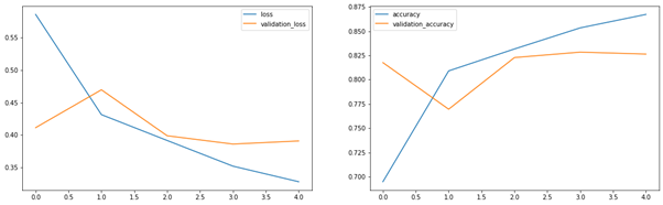
Figure 2: Train loss and validation loss curves
Conclusion
In this article, we have introduced recurrent neural nets, a class of deep neural networks, that is especially suitable when our machine learning problem involves sequences of data, such as translation of texts or predicting the prices of financial securities.
Another distinction is that they remember what they learnt from previous inputs fed to the RNN when generating predictions for the current input, which distinguishes them from normal feed forward networks which produce the output based on the current input only.
Recurrent neural nets (RNN) come in different varieties, which include, among others, the following models:
- Encoder decoder or sequence to sequence RNNs,
- Bidirectional RNNs,
- Recursive RNNs,
- Gated Recurrent Unit (GRU),
- LSTM RNNs.
One of the most popular recurrent neural nets is Long short-term Memory or LSTM neural network, which played an important role in solving the vanishing gradient problem of recurrent neural nets. LSTM is also the building block of many applications in areas of machine translation, speech recognition and other tasks, where LSTM networks achieved considerable success.