Logistic regression belongs to the class of supervised classification algorithms. It uses logistic function as a model for the dependent variable with discrete possible results.
Logistic regression can be either binary (e.g. in spam classification) or we can model multiple discrete outcomes in a variant known as multinomial logistic regression.
One way to look at logistic regression is as generalization of the linear regression, with adjustment to the classification tasks. In both regressions we are calculating the weighted sum of the input features variables and a bias term. The difference between linear and logistic regression is that in case of linear regression, this weighted sum is already the output of the model, whereas the logistic regression calculates the logistic of this weighted sum:
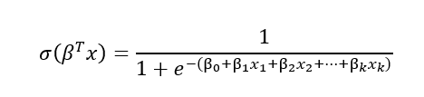
Based on this logistic value and the decision function below, we can predict the outcome:
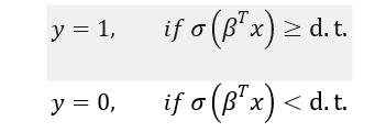
d.t. is decision threshold, which is often set at 0.5. In some cases, a different decision threshold may be warranted. Let us take a quick look at how to select decision thresholds for classification problems. The discussion is valid not only for logistic regression but also for other possible classification problems.
How to select appropriate decision threshold of logistic regression
Although machine learning practitioners often leave d.t. at 0.5, it is however important to always explore whether 0.5 is the appropriate value or some other d.t. may be more appropriate.
The key question in deciding on decision threshold is how important (relatively to each other) are false positives and false negatives in your machine learning problem. Or in other words, is it more important to have higher precision or higher recall.
Changing decision threshold of the classifier namely has an opposite effect these two important classification metrics. Precision is a metric that helps us answer how many of the positive outcomes were correct, while recall helps us in answering how many of the actual positive outcomes were correctly identified.
If we increase the decision threshold, this lowers the number of false positives, increases false negatives and thus leads to higher precision and lower recall. Conversely, if we decrease decision threshold this leads to in decrease of precision and increase in recall. This behavior is also known as precision recall tradeoff.
Different classification problems may require different combinations of precision and recall metrics.
Let us say that our classifier is used for predicting life threatening diseases. In this case, we want to lower false negatives as much as possible (this is high recall), with taking the rise of false positives (low precision) as part of the precision recall trade-off. This is actually acceptable in this context as discharging sick patient as a healthy one gives us less options to correct such a mistake than wrongly identifying healthy patients as sick. The latter error may be at some later stage corrected with further tests.
On the other hand, let us consider a classification problem where we want to identify potential new oil wells in a large oil drilling area. In this particular case, we would like to reduce the number of false positives (high precision), as initial drilling costs can be very high. If we it happens that we wrongly classify the prospect of potential oil well, there are still other oil wells available in considered region (low recall).
One approach to help us decide what decision threshold may be appropriate for our problem is to plot the ROC curve for the classification. The plot is obtained by plotting True Positive Rate, TPR=TP/(TP+FN), against the FPR, FPR=FP/(FP+TN), for different decision threshold values.
Training the logistic regression model
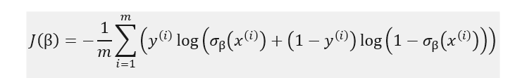
We would like a loss function to have the following feature – high probabilities for positive outcomes (y_i=1) and low probabilities for negative outcomes (y_i=0). Log loss function as defined below fits very well with this:
In the second part of our post, we will code logistic regression from scratch, using gradient descent method, so it is useful to also derive the formulas partial derivatives of the cost function:
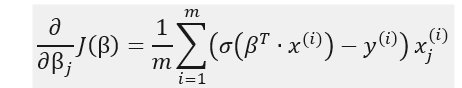
The formula indicates that the partial derivatives can be obtained by calculating for each data instance the product of the prediction error with the j-th feature value and then perform averaging over all instances.
Logistic regression regularization
When using logistic regression one sometimes encounters overfitting. This often happens when we have to model classification for a problem with a very large number of features. Besides early stopping, an efficient solution to deal with overfitting is to add a penalty to the loss function:
This leads to an additional term in the partial derivatives formula:
Logistic regression from scratch using Python
We will now show how one can implement logistic regression from scratch, using Python and no additional libraries.
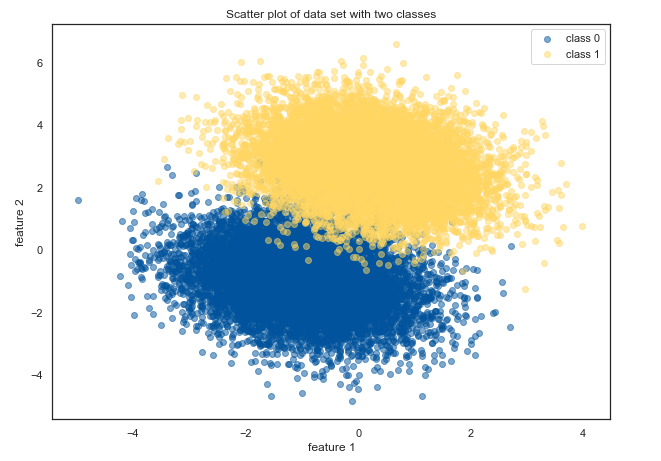
In first step, we need to generate some data. We will do this by using a multivariate normal distribution. Our model will have two features and two classes.
import numpy as np
import matplotlib.pyplot as plt
from sklearn.model_selection import train_test_split
%matplotlib inline

np.random.seed(1)
number_of_points = 10000
means = [[-1,-1],[0.2,2.7]]
cov = -0.25
covariances = [[[1,cov],[cov,1]],[[1,cov],[cov,1]]]
a = np.random.multivariate_normal(means[0],covariances[0],number_of_points)
b = np.random.multivariate_normal(means[1],covariances[1],number_of_points)
X = np.vstack((a,b))
X = np.hstack((np.ones((X.shape[0],1)),X)) # adding column of ones (biases)
y = np.array([i//number_of_points for i in range(2*number_of_points)])
X_train, X_test, y_train, y_test = train_test_split(X, y, test_size=0.2, random_state=15)

plt.figure(figsize=(10,16))
plt.subplot(2, 1, 1)
color_1='#FFD662FF'
color_0='#00539CFF'
plt.scatter(a[:,0],a[:,1],c=color_0,alpha=0.5,label='class 0')
plt.scatter(b[:,0],b[:,1],c=color_1,alpha=0.5,label='class 1')
plt.legend()
plt.xlabel('feature 1')
plt.ylabel('feature 2')
plt.title('Scatter plot of data set with two classes')
Our code generates two clusters of data with partial overlap:
Training
Next, we will define our custom Logistic Regression class:
class LogisticRegressionCustom():

    def __init__(self, l_rate=1e-5, n_iterations=50000):
        self.l_rate = l_rate
        self.n_iterations = n_iterations

    def initial_weights(self, X):
        self.weights = np.zeros(X.shape[1])

    def sigmoid(self, s):
        return 1/(1+np.exp(-s))

    def binary_cross_entropy(self, X, y):
        return -(1/len(y))*(y*np.log(self.sigmoid(np.dot(X,self.weights)))+(1-y)*np.log(1-self.sigmoid(np.dot(X,self.weights)))).sum()

    def gradient(self, X, y):
        return np.dot(X.T, (y-self.sigmoid(np.dot(X,self.weights))))

    def fit(self, X, y):
        self.initial_weights(X)
        for i in range(self.n_iterations):
            self.weights = self.weights+self.l_rate*self.gradient(X,y)
            if i % 10000 == 0:
                print("Loss after %d steps is: %.10f " % (i,self.binary_cross_entropy(X_test,y_test)))
        print("Final loss after %d steps is: %.10f " % (i,self.binary_cross_entropy(X_test,y_test)))
        print("Final weights: ", self.weights)
        return self

    def predict(self, X):
        y_predict = []
        for t in X:
            y_predict.append(1) if self.sigmoid(np.dot(self.weights,t))>0.5 else y_predict.append(0)
        return y_predict

    def predict_proba(self, X):
        y_predict = []
        for t in X:
            y_predict.append(self.sigmoid(np.dot(self.weights,t)))
        return y_predict
We can then run the training of our model:
lr = LogisticRegressionCustom()
lr.fit(X_train,y_train)
After training, we obtain the following weights of our custom logistic regression model:
Final weights: [-2.87044201 2.27853577 4.42372951]
Inspecting incorrectly classified instances
To estimate the performance our logistic regression model, we can plot the instances and visually denote the points that were incorrectly classified (they are denoted with red):
def colors(s):
    if s == 0:
        return color_0
    elif s == 1:
        return color_1
    else:
        return 'coral'

plt.figure(figsize=(10,16))
y_predict = lr.predict(X_test)
classify = []
for i,p in enumerate(y_predict):
    if y_predict[i] == y_test[i]:
        classify.append(y_predict[i])
    else:
        classify.append(2)

plt.subplot(2, 1, 2)
plt.xlabel('feature 1')
plt.ylabel('feature 2')
plt.title("Scatter plot of test instances (misclassified points denoted with red)")
for i,x in enumerate(X_test):
    plt.scatter(x[1],x[2],alpha=0.5,c=colors(classify[i]))
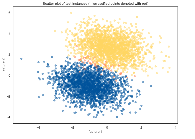
Misclassified data points (denoted in image above as red) are somehow expectedly either near the boundary between both classes or in the area of the opposite class.
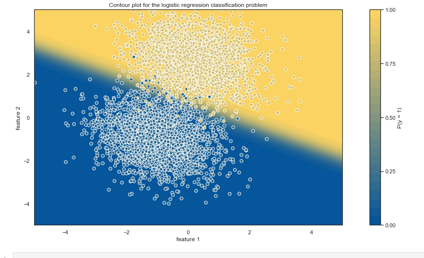
We can gain further insights by generating contour plot:
import numpy as np
import seaborn as sns
import matplotlib.colors

sns.set(style="white")
N=1000
x_values=np.linspace(-5.0, 5.0, N)
y_values=np.linspace(-5.0, 5.0, N)
x_grid, y_grid=np.meshgrid(x_values, y_values)
grid_2d=np.c_[x_grid.ravel(), y_grid.ravel()]
new=[[1]+i for i in grid_2d.tolist()]
classes=np.array(lr.predict_proba(new)).reshape(x_grid.shape)

norm = matplotlib.colors.Normalize(0,1)
colors = [[norm( 0), color_0],
          [norm( 1.0), color_1]]

cmap = matplotlib.colors.LinearSegmentedColormap.from_list("", colors)

fig,ax=plt.subplots(figsize=(20, 8))
cs=ax.contourf(x_grid, y_grid, classes, 25, cmap=cmap, vmin=0, vmax=1)
cbar=fig.colorbar(cs)
cbar.set_label("P(y = 1)")
cbar.set_ticks([0, 0.25, 0.5, 0.75, 1])
plt.title("Contour plot for the logistic regression classification problem")

ax.scatter(X_test[:,1],X_test[:,2],c=y_test[:],s=40,cmap=cmap,vmin=-.25,vmax=1.25,
           edgecolor="white",linewidth=1)

ax.set(aspect=0.7, xlim=(-5, 5), ylim=(-5, 5), xlabel="feature 1", ylabel="feature 2")
Comparison of our custom logistic regression and results obtained by using scikit-learn
To assess our results that we obtained with logistic regression from scratch, we will compare it with those obtained with Logistic Regression as implemented in the scikit-learn library.
Our logistic regression from library did not use regularization, so we will set sklearn regularization parameter C for the logistic regression to a very high value (note that 1/C measures the regularization strength).
from sklearn.linear_model import LogisticRegression
from sklearn.metrics import log_loss
model = LogisticRegression(C=1e5, solver = 'saga', fit_intercept=False)
model=model.fit(X_train, y_train)
y_pred=model.predict(X_test)

y_pred = model.predict_proba(X_test)
print('Weights: ',model.coef_[0])
print('Logloss: ',log_loss(y_test,y_pred))
The following table shows the comparison of weights and logloss from both approaches, logistic regression from scratch and sklearn implementation:
| Method | Weights vectors | Loss |
| Logistic regression from scratch | [-2.87044201 2.27853577 4.42372951] | 0.041164327 |
| Logistic regression with sklearn | [-2.87047406 2.27860591 4.4237207 ] | 0.041164038 |

Get in Touch
Do you need consultation or have a project in mind? We would love to hear from you!


0 Comments