Decision trees are algorithms with tree-like structure of conditional statements and decisions. They are used in decision analysis, data mining and in machine learning, which will be the focus of this article.

In machine learning, decision trees are both excellent models when used on their own as well as when used for more advanced methods such as random forests and gradient boosting machines.

Decision tree are supervised machine learning models that can be used both for classification and regression problems. They are commonly referred to as CART (Classification and Regression Trees).

“The possible solutions to a given problem emerge as the leaves of a tree, each node representing a point of deliberation and decision.” Niklaus Wirth (1934 — )

Decision trees have a tree-like partition (see Fig. 1), consisting of:

decision nodes which split into two or more branches,
leaf or terminal nodes which represent end of branches (and are not split further).

The node at the top of the decision tree is called root node and represents the best predictor.

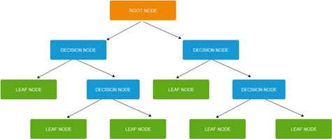
Figure 1: Decision tree

Decision trees are built or grown by finding at each decision node the feature that best separates the data into subsets that are most homogenous. This procedure is used recursively until classification can be achieved for each leaf of the decision tree.

Large decision trees are prone to overfitting or performing poorly on generalization to new, unseen samples. One method of regularizing decision trees is by controlling their size.

It is hard to tell during building of the decision tree at what level should the algorithm stop. The most common approach to controlling the size of decision tree is thus to grow the tree to a size where nodes have only a small number of instances. After the tree is grown, it is then pruned by removing nodes which do not provide predictive value.

Pruning can start at the root level or is applied bottom to top. An example of the latter approach is reduced error pruning, which starts at leaves with each node replaced with its most popular class.

Decision tree inference for data instances is done by following the tree from the root node, testing the appropriate attribute at each decision node until reaching a leaf node and determining the corresponding classification or regression result.

Growing the decision trees

In growing the decision tree, the most important task is deciding which attribute or feature best splits the data into most homogenous subsets at each node.

There are different metrics that we can use to measure the optimality of node splits: Gini impurity, Information gain and Variance reduction.

Gini impurity

Gini impurity measures the likelihood of wrong classification of a new data point, randomly chosen from the set, if this new data point was randomly labelled according to the distribution of labels in the data set. Gini impurity is calculated with the following formula:

where p_i is fraction of instances labelled with class i in the data set.

Information gain

Information gain is based on the concept of entropy, which in our case measures the degree of homogeneity in group of data points.

Entropy can be calculated with:

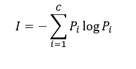
where P_i is proportion of data that belong to class i. Entropy is 0 if all samples belong to the same class and is large when proportions for different classes are equal (see Fig. 2).

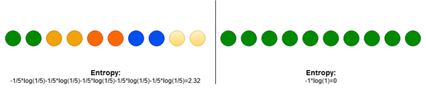
Figure 2: Entropy for two different distributions

In context of decision trees, information gain measures the change in entropy after we split the data set on specific attribute.

We calculate information gain by determining weighted entropies of each branch and subtracting it from the initial entropy. Splits that result in the most homogenous branches deliver the highest information gain.

Information gain is used by ID3, C4.5 and C5.0 tree building algorithms.

Variance reduction

Variance reduction is usually applied when considering a regression problem. In this approach, the best splits are those which most decrease the combined weighted variance of child nodes

In most cases for CART problems, Gini impurity and Information gain deliver very similar results. Gini impurity does however have an advantage over Information gain in being slightly faster, as there is no need for log calculations.

Decision Tree Algorithms

Decision trees can be built with many different algorithms, including:

ID3,
CART,
5,
Chi-square automatic interaction detection (CHAID).

ID3 algorithm

ID3 (Iterative Dichotomiser 3) algorithm trains the decision trees using a greedy method. On each step, the algorithm calculates entropies of unused attributes. It then selects the attribute with the smallest entropy, i.e. largest information gain. Recursion of algorithm stops when all the attributes have been used or all data points have been classified.

Regularizing decision trees

Decision tree is an example of a non-parametric machine learning model. Non-parametric machine models are not without parameters, the number of its parameters grows with the number of data instances and can often be much larger than in the case of parametric models.

This gives the non-parametric models such as decision trees much more space to closely fit the train data set, often leading to overfitting. To avoid the latter, one can apply regularization and limit the decision trees when training.

One regularization method is to restrict the maximum depth of the decision tree. Other parameters that can be regularized include:

minimum samples a node must have before it can be split
minimum number of samples a leaf node must have
maximum number of leaf nodes
maximum number of features

Advantages and Disadvantages of Decision Trees

Decision trees have many important advantages:

high interpretability – they are easy to understand and interpret, which is an important feature in view of recent rise in importance of Explainable Artificial Intelligence (XAI),
they can be applied on problems that have both continuous and categorical data,
decision trees are less demanding in terms of data preparation,
they can be used on large data sets, obtaining a decent performance,
they have in-built feature selection.

Decision trees also have several limitations:

they have high variance, i.e. small variations in training data can lead to large changes in resulting tree structure and inference results. Variance of decision trees can be reduced with boosting and bagging methods,
decision trees are non-parametric methods, where the number of parameters grows with size of train data set. This can lead to large and complex decision trees that are prone to overfitting,
decision tree algorithms are greedy with locally optimal choices being made at each decision node. The result of training may thus be decision trees that are not globally optimal.

In the second part of our article, we will build a decision tree model for prediction of heart disease.

Heart disease prediction with decision tree

We will be working with the Heart Disease Data set, available at UCI machine learning repository:

https://archive.ics.uci.edu/ml/datasets/heart+Disease

As part of data preparation, we will rename some columns in the original data, set descriptive values for categorical features and consolidate status of heart diseases (1,2,3,4 to 1), so that our target variable has two values: 0 (no heart disease) and 1 (having a heart disease). We will also remove 6 rows with missing values.

import pandas as pd

from sklearn.model_selection import train_test_split

from sklearn.metrics import classification_report,confusion_matrix,accuracy_score

from sklearn.tree import DecisionTreeClassifier

import matplotlib.pyplot as plt

import numpy as np

import seaborn as sns

from graphviz import Source

from sklearn import tree

from IPython.display import SVG

import scipy.stats as sstats

missing_values = ["?"]

df = pd.read_csv('processed.cleveland.csv',header=None,na_values = missing_values)

df.columns = ['age','sex','chest_pain_type','resting_blood_pressure','serum_cholestoral','fasting_blood_sugar','resting_electrocardiographic',

           'maximum_heart_rate','exercise_induced_angina','ST_depression','slope_of_peak_exercise','number_major_vessels','thalassemia','target']

df.dropna(inplace=True)

df['target'] = df['target'].map({0:0,1:1,2:1,3:1,4:1})

df['sex'] = df['sex'].map({0:'female',1:'male'})

df['chest_pain_type'] = df['chest_pain_type'].map({1:'typical angina',2:'atypical angina',3:'non-anginal pain',4:'asymptomatic'})

df['fasting_blood_sugar'] = df['fasting_blood_sugar'].map({1:'fasting blood sugar greater than 120 mg/dl',0:'fasting blood sugar less than 120 mg/dl'})

df['resting_electrocardiographic'] = df['resting_electrocardiographic'].map({0:'normal',1:'ST-T wave abnormality',2:'left ventricular hypertrophy'})

df['exercise_induced_angina'] = df['exercise_induced_angina'].map({0:'no',1:'yes'})

df['slope_of_peak_exercise'] = df['slope_of_peak_exercise'].map({1:'upsloping',2:'flat',3:'downsloping'})

df['thalassemia'] = df['thalassemia'].map({3:'normal',6:'fixed defect',7:'reversable defect'})

Plotting the distribution of patients with respect to disease status shows us that both classes are roughly equally balanced:

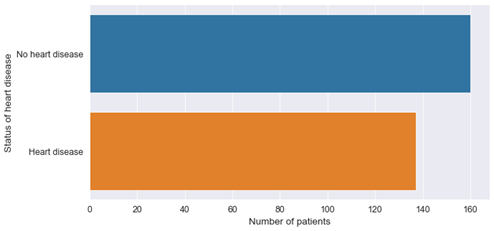
Figure 3: Balance in data set

target_variable_name='target'

plt.figure(figsize = (10, 5))

ax = sns.countplot(y=target_variable_name, data=df)

ax.set_title("Heart disease/No heart disease");

ax.set_xlabel("Number of pateients");

ax.set_ylabel("Status of heart disease");

ax.set_yticklabels(labels=['No heart disease','Heart disease'])

Pearson correlations between numerical features (see Fig. 4) indicate that numerical features have relatively low correlation.

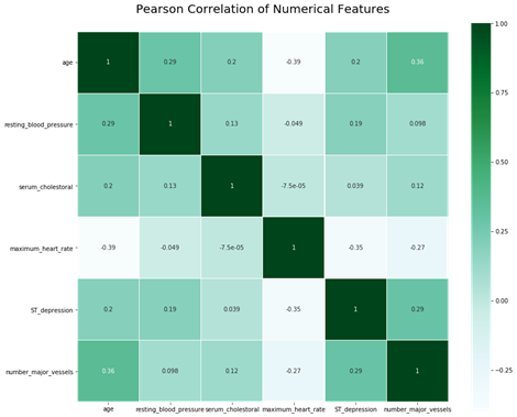
Figure 4: Correlation of numerical features

plt.figure(figsize=(14,12))

target_variable_name = 'target'

numerical_features = ['age','resting_blood_pressure','serum_cholestoral','maximum_heart_rate','ST_depression','number_major_vessels']

plt.title('Pearson Correlation of Numerical Features', y=1.04, size=20)

sns.heatmap(df[numerical_features].astype(float).corr(),linewidths=0.15,square=True, vmax=1.0, cmap=plt.cm.BuGn, linecolor='white', annot=True);

In examining correlation of categorical features, we could in principle use one hot encoding, however, the analysis would be difficult due to the large number of resulting features.

A better approach is to use implementation of Cramér’s V with biased correction (see also: Bergsma, Wicher, 2013, “A bias correction for Cramér’s V and Tschuprow’s T”. Journal of the Korean Statistical Society and discussion).

Correlation between categorical features are also relatively low (see Fig.5).

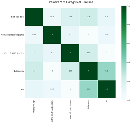
Figure 5: Correlation of categorical features

categorical_features = ['chest_pain_type','resting_electrocardiographic','slope_of_peak_exercise','thalassemia']

def cramers_v_with_bias_correction(x, y):

    cm = pd.crosstab(x,y).values

    chi2 = sstats.chi2_contingency(cm)[0]

    cm_sum = cm.sum().sum()

    phi2 = chi2/cm_sum

    r,k = cm.shape

    phi2corr = max(0, phi2-((k-1)*(r-1))/(cm_sum-1))

    rcorr = r-((r-1)**2)/(cm_sum-1)

    kcorr = k-((k-1)**2)/(cm_sum-1)

    return np.sqrt(phi2corr/min((kcorr-1),(rcorr-1)))

cramers_v = np.zeros((len(categorical_features),len(categorical_features)))

for i,feature1 in enumerate(categorical_features):

    for j,feature2 in enumerate(categorical_features): 

        cramers_v[j,i] = cramers_v_with_bias_correction(df[feature1],df[feature2])

cramers_v = pd.DataFrame(cramers_v,index=categorical_features,columns=categorical_features)


plt.figure(figsize=(14,12))

plt.title("Cramér's V of Categorical Features", y=1.04, size=20)

sns.heatmap(cramers_v,linewidths=0.15,square=True, vmax=1.0, cmap=plt.cm.BuGn, linecolor='white', annot=True);

Based on determined correlations, we will not remove any features from our initial selection. We next examine distribution plots for numerical features (see Fig. 6).

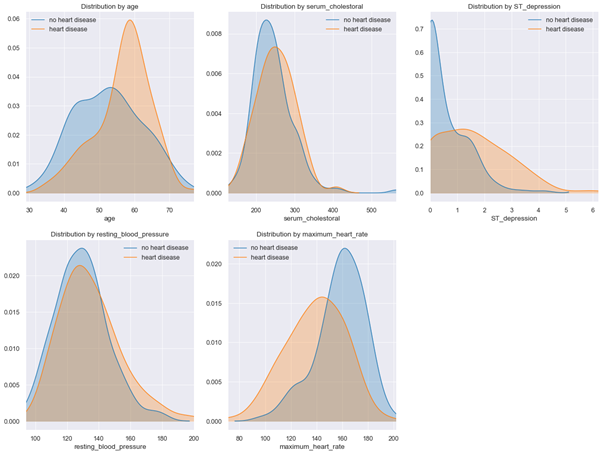
Figure 6: Distribution plots for numerical features

Kernel density plots show that patients with heart disease have a slightly higher resting blood pressure, are older on average, have higher serum cholesterol levels and lower maximum heart rates under stress test.

Additional insights can be obtained by plotting distribution for categorical features (see Fig. 7):

fig, axes = plt.subplots(nrows=2, ncols=2,figsize=(20,15))

for index,feature in enumerate(categorical_features):

    x = index % 2 

    y = index // 2      

    df1 = df.groupby([feature,'target'], sort=False).size().unstack(fill_value=0)

    df1.columns = ['No Heart Disease','Heart Disease']

    values_0 = df1['No Heart Disease'].values

    values_1 = df1['Heart Disease'].values

    indices = range(len(df1.index.values))

    axes[x,y].bar(indices, values_0, width, label='No Heart Disease')

    axes[x,y].bar(indices, values_1, width,bottom=values_0,label='Heart Disease')

    axes[x,y].set_xticks(indices)

    axes[x,y].set_xticklabels(tuple(df1.index.values))

    axes[x,y].set_ylabel('Number of patients')

    axes[x,y].set_title('Distribution for '+feature)

    axes[x,y].legend()

The data indicate that proportion of healthy patients with no heart disease is higher among patients that have:

normal thalassemia,
chest pain type of non-anginal pain,
number of major vessels equal to 0,
are female,
have upsloping peak exercise slope.

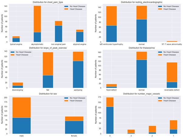
Figure 7: Distribution plots for categorical features

We will now train a decision tree on the heart disease data set. We would expect that the attributes on which the decision tree will be optimally split during growing can be found among the attributes that we just highlighted with the help of distribution analysis.

Training a decision tree classifier

We will use Scikit-learn library to build a decision tree classifier, the maximum depth to which the tree can grow will be set to 3.

First, we will use function get_dummies from pandas to one hot encode the categorical features:

df = pd.get_dummies(df,drop_first=True)

Next, we prepare the train and test data and train the decision tree:

X = df.copy(deep=True)

y = X['target']

del X['target']

X_train, X_test, y_train, y_test = train_test_split(X,y,test_size=0.20, random_state=4)

dt = DecisionTreeClassifier(random_state=0,max_depth=3)

dt.fit(X_train,y_train)

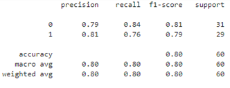
Our decision tree achieves 80% accuracy on the test set:

y_pred = dt.predict(X_test)

print(classification_report(y_test,y_pred))

Confusion matrix with recall rates:

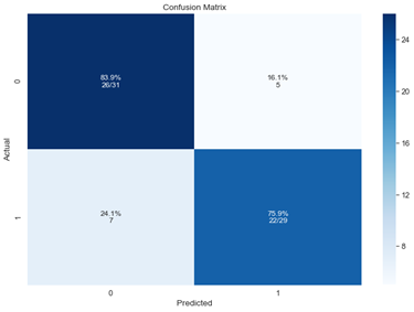
Figure 8: Confusion matrix

Finally, we can visualize our grown decision tree (Fig. 9):

graph = Source( tree.export_graphviz(dt, out_file=None,filled=True, feature_names=X_train.columns))

SVG(graph.pipe(format='svg'))

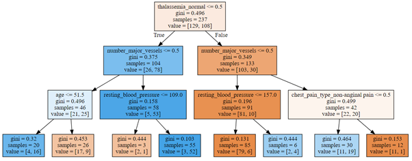
Figure 9: Decision tree for prediction of heart disease

The best predictor is the attribute thalassemia_normal and the first splitting is performed by checking if thalassemia is normal or not. The second node is split on variable number of major vessels, followed in the next level by splitting on age, resting blood pressure and chest pain type of non-anginal pain.

In terms of splitting attributes, our decision tree is thus very similar to a decision tree that we would build based on our earlier analysis, which considered only distribution of patients for different attributes.

Decision trees with python