There are many complex and almost instantaneous ad processes that happen when we visit a typical website. The ads that we see on websites are selected in less than 100 milliseconds through specialized auctions in which advertisers bid on ad impressions and publishers sell them.

An important part of optimal bidding strategies in these ad auctions involves calculation of bid prices based on estimated click-through-rate (CTR) for given ad impression. CTR prediction is thus one of the key methods in the RTB ecosystem.

In this article, we will build two machine learning models for predicting whether an ad will be clicked or not. We will use a data set from a Kaggle competition by Avazu – “Click-Through Rate Prediction”, available at https://www.kaggle.com/c/avazu-ctr-prediction. It contains 11 days worth of ad clicks data.

Features in our data set consist of:

– id: ad identifier

– hour: format is YYMMDDHH, so 14091123 means 23:00 on Sept. 11, 2014 UTC.

– C1 — anonymized categorical variable

– banner_pos

– site_id

– site_domain

– site_category

– app_id

– app_domain

– app_category

– device_id

– device_ip

– device_model

– device_type

– device_conn_type

– C14-C21 — anonymized categorical variables

– click, 0 for non-click, 1 for click (our target variable column)

Before using the data set for training, we shuffle its rows (using bash command “shuf -o train_shuffled.csv < train.csv”).

We start by importing the libraries:

import pandas as pd

import numpy as np

import matplotlib.pyplot as plt

import seaborn as sns

import datetime

import scipy.stats as sstats

import csv

import numpy as np

import pandas as pd

from datetime import datetime, date, time

from sklearn.linear_model import SGDClassifier

from sklearn.metrics import log_loss

from sklearn.feature_extraction import FeatureHasher

from sklearn import preprocessing

from sklearn.pipeline import Pipeline

from sklearn.externals import joblib

from fastFM.mcmc import FMClassification

from sklearn.preprocessing import OneHotEncoder

To better understand our data set we will first load 100,000 rows for initial exploratory data analysis:

dataset = r'train_shuffled.csv' 

df = pd.read_csv(dataset,nrows=100000)

df = df.drop('id', axis=1)

# we do not need column id

Let us first examine the imbalance in our data set:

print("Imbalance ratio: {}".format(float(len(df[df['click']==0]))/len(df[df['click']==1])))

Imbalance ratio: 4.87

Our data set displays some imbalance with ads that were not clicked representing the majority of data instances.

Next, we calculate the CTR in our ads sample:

print("CTR is {}%".format(100.0*df['click'].sum()/len(df)))

CTR is 17.144%

Prior to training, we perform feature engineering, but restricted on datetime column:

df['hour']=df['hour'].map(lambda x: datetime.strptime(str(x),"%y%m%d%H"))

df['day_of_week']=df['hour'].map(lambda x:  x.weekday())

df['hour']=df['hour'].map(lambda x:  x.hour)

Next, we want to qualitatively examine the CTR for different features, but we will limit visualizations to categorical features that do not have too many distinct values and are not anonymized.

df.nunique()

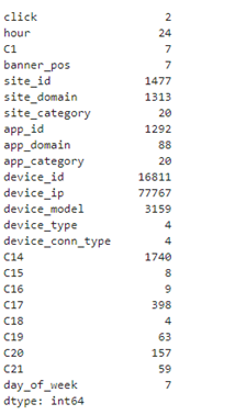
Based on number of unique values, we visually examine CTR of the following features:

highlighted_features = ['banner_pos','device_type', 'device_conn_type','day_of_week','hour']

sns.set_context("paper",font_scale=1.3)

sns.set_style("darkgrid")

width = 0.35

fig, axes = plt.subplots(nrows=2, ncols=2,figsize=(20,15))

for index,feature in enumerate(highlighted_features[:len(highlighted_features)-1]):

    x = index // 2 

    y = index % 2      

    df1 = df.groupby([feature,'click'], sort=True).size().unstack(fill_value=0)

    df1.columns = ['not clicked','clicked']

    indices = range(len(df1.index.values))

    ctr = [float(value)/(df1['not clicked'].values[i] + value) for i,value in enumerate(df1['clicked'].values)]

    axes[x,y].bar(indices, df1['not clicked'].values, width, label='not clicked')

    axes[x,y].bar(indices, df1['clicked'].values, width,bottom=df1['not clicked'].values,label='clicked')

    axes[x,y].set_xticks(indices)

    axes[x,y].set_xticklabels(tuple(df1.index.values))

    axes[x,y].set_ylabel('Number of ads / CTRs')

    axes[x,y].set_title('CTR for '+feature)

    axes[x,y].legend() 

    for p in  axes[x,y].patches:

        if p.get_height() in df1['not clicked'].values: 

            axes[x,y].annotate('CTR='+format(100*ctr[np.where(df1['not clicked'].values == p.get_height())[0][0]], '.1f')+'%', (p.get_x() + p.get_width() / 2., p.get_height()*1.2 ), ha = 'center', va = 'center', 

                                   xytext = (0, 10), textcoords = 'offset points')

plt.show()

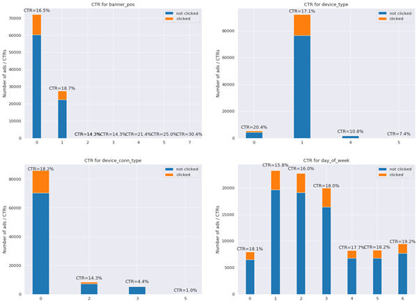
Figure 1: CTR for different feature values

Charts show that there is a considerable difference between click-through-rates depending on device type, device connection type and banner position. CTR is also not uniform with respect to the day of week on which the ad is clicked.

Analysing CTR for different hours of the day:

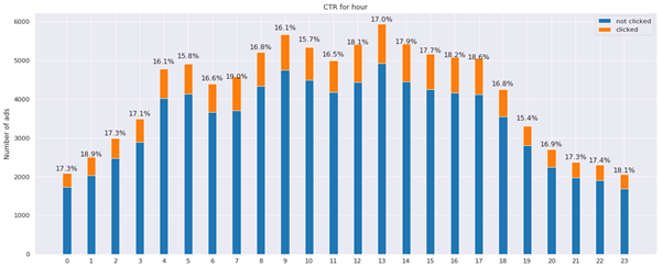
Figure 2: CTR for different hours of the day

Certain hours of the day, like 1, 7, 17 exhibit higher CTR than average, though they are not clustered together. Lower CTR than average is on the other hand registered in the hours between 17 and 19.

Next, we examine correlation between categorical features, using Cramer’s V measure for this purpose:

categorical_features = highlighted_features

def cramers_v_with_bias_correction(x, y):

    cm = pd.crosstab(x,y).values

    chi2 = sstats.chi2_contingency(cm)[0]

    cm_sum = cm.sum().sum()

    phi2 = chi2/cm_sum

    r,k = cm.shape

    phi2corr = max(0, phi2-((k-1)*(r-1))/(cm_sum-1))

    rcorr = r-((r-1)**2)/(cm_sum-1)

    kcorr = k-((k-1)**2)/(cm_sum-1)

    return np.sqrt(phi2corr/min((kcorr-1),(rcorr-1)))

cramers_v = np.zeros((len(categorical_features),len(categorical_features)))

for i,feature1 in enumerate(categorical_features):

    for j,feature2 in enumerate(categorical_features): 

        cramers_v[j,i] = cramers_v_with_bias_correction(df[feature1],df[feature2])

cramers_v = pd.DataFrame(cramers_v,index=categorical_features,columns=categorical_features)

plt.figure(figsize=(14,12))

plt.title("Cramer's V of Categorical Features", y=1.04, size=20)

sns.heatmap(cramers_v,linewidths=0.15,square=True, vmax=1.0, cmap=plt.cm.BuGn, linecolor='white', annot=True);

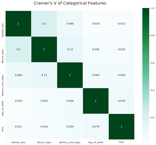
Figure 3: Cramer’s V of categorical features

When looking at non-anonymized features, correlations are rather low, except between device type and banner position.

2. CTR-prediction using SGD and hashing trick

After introduction to our data sets, we will next build our first model to predict whether a given ad will be clicked by the user or not. Our Avazu data set consists of around 40 million rows, the corresponding .csv file has a size of 6GB.

We will treat our problem as out-of-core learning, where we will not load entire train data set in memory. We will rather input and process data on a row by row basis, each time updating weights of our ML model.

Stochastic Gradient Descent

To achieve this online learning, we will use Stochastic Gradient Descent method with updates to the model done for a single data instance at a time. Scikit-learn has several excellent online learning algorithms available, we will be using SGDClassifier.

SGDClassifier has a complexity of O(knp), where k is the number of epochs, p is the average number of non-zero features per sample and n is the number of data instances. SGDClassifier time complexity thus increases linearly with training data size. Another advantage is fixed memory footprint, making it highly scalable.

In order to use SGDClassifier as out-of-core learner, we must use the method partial_fit instead of fit. To use partial_fit, we need to parse through the entire data set at least once to determine the classes that we want to predict. These classes should be passed to partial_fit under parameter classes. In our case, we only have two of them – 0 and 1.

Hashing trick or feature hashing

Categorical features in our data set have millions of unique values. In order to manage this high cardinality, we will use feature hashing or hashing trick approach. Feature hashing maps sparse, high-dimensional features to smaller vectors of fixed size.

It is very useful in out-of-core learning as it does not require us to parse the complete data set. It computes feature indices directly from feature values, using a hashing function. One can use different hashing functions, good hashing functions however have the following properties:

• hash value is completely determined by the input value
• the resulting hash values are mapped as uniformly as possible across hash value space
• hashing function uses all the input data
• the same input value always produces the same hash value (deterministic)

When the dimension of hashing vector is smaller than the initial feature space, the hashing function can hash different input values to the same hash value, known as “collision”. Many studies however show that impact of collisions on predictive performance of models is limited, see e.g. https://arxiv.org/pdf/0902.2206.pdf.

Although feature hashing has several advantages, it also has some drawbacks. One is that we need to explicitly set the hashing space size. Another drawback is reduced interpretability of models that use feature hashing. This is a consequence of loss of information on application of hashing function. Although the same input feature values lead to the same hash value, we cannot perform reverse lookup and determine the exact input feature value from the hash value.

This means that when we determine the most important features for predictions of our model using e.g. XAI (Explainable AI) tools like SHAP and LIME, we will have difficulty in mapping these features to those in the initial feature set. Application of feature hashing may thus lead to lower interpretability of our model.

Feature hashing is implemented in several open source machine learning tools, such as Vowpal Wabbit and Scikit-learn. In our training, we will use FeatureHasher from scikit-learn.

Let us start by defining several variables and the SGD model:

train_file = dataset 

chunk_size = 100000

train_size = 0.8

total_rows = 40428967

train_rows = int(train_size*total_rows)

test_rows = total_rows - train_rows

nr_iterations_train = round(train_rows/chunk_size)

nr_iterations_test = round(test_rows/chunk_size)

SGDmodel = SGDClassifier(loss='log',  alpha=.000001, penalty='l2', eta0=2.0, shuffle=True, n_jobs=-1,learning_rate='invscaling',  random_state=10)

partial_fit_classes = np.array([0, 1]) # to be used in partial_fit method

Defining instance of FeatureHasher:

h = FeatureHasher(n_features=2**26, input_type='string')

preprocessor = Pipeline([('feature_hashing', h)])

 

Setting up readers of data:

columns = ['id', 'click', 'hour', 'C1', 'banner_pos', 'site_id', 'site_domain', 'site_category', 'app_id', 'app_domain', 'app_category',

           'device_id', 'device_ip', 'device_model', 'device_type', 'device_conn_type', 'C14', 'C15', 'C16', 'C17', 'C18', 'C19', 'C20', 'C21']

df_train = pd.read_csv(

    train_file, sep=',', chunksize=chunk_size, names=columns, header=0, nrows=train_rows)

df_test = pd.read_csv(train_file, sep=',',

                        chunksize=chunk_size, names=columns, header=0, skiprows=train_rows, nrows=test_rows)

 

Defining function for pre-processing of data instances:

def preprocess_data(df):

    y_train = df['click'].values

    y_train = np.asarray(y_train).ravel()

    df['hour'] = df['hour'].map(

        lambda x: datetime.strptime(str(x), "%y%m%d%H"))

    df['day_of_week'] = df['hour'].map(lambda x:  x.weekday())

    df['hour'] = df['hour'].map(lambda x:  x.hour)

    X = df.drop(['id', 'click'], axis=1)

    X_train = preprocessor.fit_transform(np.asarray(X.astype(str)))

    return y_train, X_train

 

Starting the training:

print("Training...")

count = 0

logloss_sum = 0

for df in df_train:

    count += 1

    y_train, X_train = preprocess_data(df)

    SGDmodel.partial_fit(X_train, y_train, classes=partial_fit_classes)

 

Followed by computing log loss on test set:

print("Log loss on test set ...")

logloss_sum = 0

count = 0

for df in df_test:

    count += 1

    y_test, X_test = preprocess_data(df)

    y_pred = SGDmodel.predict_proba(X_test)

    log_loss_temp = log_loss(y_test, y_pred)

    logloss_sum += log_loss_temp

    if count % 10 == 0:

        print("Iteration {}/{}, test log loss: {}".format(count,nr_iterations_test,logloss_sum/count))

print("Final log loss: ", logloss_sum/count)

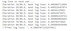
We obtain final log loss of 0.3995.

3. Factorization Machines

One of the most popular machine learning models for CTR prediction are Factorization Machines (FM) and its later variants, including Field Aware Factorization Machines (FFM). Factorization machines are a supervised machine learning algorithm, capable of both regression and classification, introduced by Steffen Rendle in https://www.csie.ntu.edu.tw/~b97053/paper/Rendle2010FM.pdf.

They are a generalization of a linear model and can capture higher order interactions between features. One approach to modelling higher order interactions would be to introduce mixed polynomial terms in a model known as Poly2 but that model is a O(n**2) problem which makes it prohibitively expensive both in terms of memory and time when applied on typical CTR data sets.

Rendle’s Factorization Machines reduce the polynomial calculation time to linear complexity. The interaction between features is modelled with terms of the form W_ij*x_i*x_j, where W_ij is modelled as the inner product of k-dimensional latent vectors associated with each feature. The FM approach learns these k-dimensional latent vectors for each feature, where k is a hyperparameter that must be specified by the user before the start of the training.

We replaced the learning of nXn interaction parameters with learning nXk parameters, making the problem linear in n. Or in matrix terms, instead of having a term x_transpose A x with A unconstrained (with nXn possible values), we constrain the matrix A to a form V_transpose*V with V of dimension nXk.

Factorization Machines are especially suitable for CTR predictions, where they can learn the users click rate behaviour when ads from specific categories are shown on webpages from specific categories (interaction).

There are several libraries with implementation of Factorization Machines:

• http://www.libfm.org/ (from Steffen Rendle)
• https://github.com/ibayer/fastFM

Factorization Machines are usually trained by using one of the three main solvers – Stochastic Gradient Descent (SGD), Alternative Least Squares (ALS) or Markov Chain Monte Carlo (MCMC).

We trained our Factorization Machine model using fastFM tool (with Markov Chain Monte Carlo – MCMC method), on a sample of 1 million rows from Avazu data set:

rank = 9 # the number of hidden variables per feature, selected with hyperparameter tuning

n_iter = 12 # selected with hyperparameter tuning

df = pd.read_csv(dataset,nrows=1000000)

train_size = 0.8

train_size = int(train_size*len(df))

def fast_fm(trainX, testX, trainY, testY):

    encoder = OneHotEncoder(handle_unknown='ignore').fit(trainX)

    trainX = encoder.transform(trainX)

    testX = encoder.transform(testX)

    clf = FMClassification(rank=rank, n_iter=n_iter)

    predictions = clf.fit_predict_proba(trainX, trainY, testX)

    print("fast fm log loss: ", log_loss(testY, predictions))

    return True

trainX = df.iloc[:train_size, ~df.columns.isin(['click'])]

trainY = df['click'].values[:train_size]

testX = df.iloc[train_size:, ~df.columns.isin(['click'])]

testY = df['click'].values[train_size:]

fast_fm(trainX, testX, trainY, testY)

 

Log loss of resulting Factorization Machines model is 0.4022.

Conclusion

Real time bidding (RTB) are automated digital auctions that allow advertisers to bid on ad impressions and publishers to sell them.  An important part in these ad auctions involves calculation of bid prices which often rely on estimation of click-through-rates (CTR) for given ad impression. CTR prediction is thus one of the key methods in the RTB ecosystem.

In our article, we have trained several machine learning models to predict clicks on ads, using data set from Avazu, consisting of 11 days worth of click ads. We examined two ML models, first was an out-of-core, online learner based on Stochastic Gradient Descent using feature hashing. The second model was based on Factorization Machines. This class of models and its later variants such as Field Aware Factorization Machines are among the most popular models for CTR prediction.