Natural language processing (NLP) – text pre-processing, feature extraction and word embeddings

Natural language processing (NLP) is a multi-disciplinary field of computer science, artificial intelligence and linguistics that focuses on the interaction between computers and human language, with the emphasis on the understanding, generating, manipulating and analysing human languages.

Historically, early NLP systems often relied on sets of rules, e.g. for stemming of words. Since the mid-1990s, this rule-based approach was gradually replaced with a statistical one, based on machine learning.

Natural language processing powers a wide and diverse range of today’s solutions, including:

machine translation, which is considered one of the great successes of AI in recent years and implemented in a wide range of solutions, including digital assistants,
topic modelling, helping us discover hidden topics in collections of documents,
Text summarization, which produces a concise summary of the text while still retaining its main informational value,
sentiment analysis, which is invaluable as part of opinion mining, helping companies and organizations extract opinions and sentiment expressed about their products, services by their customers or other stakeholders,
named entity recognition, an information extraction task of finding and classifying named entities in unstructured texts, where named entities can consist of persons’ names, organizations, places, expressions of times, and others,
automated question answering, a subfield which concerns itself with systems that can automatically answer questions that are asked by humans,
speech recognition, which is a multi-disciplinary field of technologies which allow computers to transform speech into texts,
document indexing, which is the method of attaching or tagging documents with additional information to help with later search or document retrieval.

Natural language processing is considered a difficult problem in artificial intelligence and computer science. This is mainly due to many different ambiguities of human languages, including lexical ambiguity or the ambiguity of single words, syntactic ambiguity, attachment ambiguity and others.

Text pre-processing

Machine learning algorithms require input data to be in a numerical format. When our input data are collections of texts, we thus first need to transform texts in the appropriate numerical form.

To prepare texts for this transformation, we apply several pre-processing steps, where the specific methods used depend on the domain and type of the machine learning algorithm used.

Some of the most common pre-processing techniques applied on texts include:

lowercasing,
removal of punctuations,
removal of special characters,
removal of stop words,
removal of frequent words,
removal of rare words,
removing numbers,
removal of emojis/emoticons or their conversion to words (if present, e.g. in tweets),
removal of URLs,
expanding contractions, (e.g. “aren’t” to “are not”),
removing misspelled words,
stemming or reducing words to their word stem or root form,
normalization, e.g. “gooood” to “good”, often used when dealing with social media comments and other “noisy” texts,
lemmatization or determining the lemma of the word.

Text pre-processing should not be indiscriminately applied to all machine learning problems. In problems involving deep neural networks which can learn complex patterns in texts, it is e.g. often better to skip stemming, lemmatization and stop words removal during text pre-processing.

Feature extraction

After pre-processing, the next step is the conversion of textual data into a numerical form which can be understood by algorithms. This mapping of text to numerical vectors is also known as feature extraction.

Bag of words

One of the simplest methods for numerical representations of texts is the bag of words (BOW). Let us take a corpus consisting of two sentences:

“I am driving a car.”

“car is parked.”

BOW approach consists of first forming a vocabulary consisting of unique words present in documents of the corpus, in our case: (“I”, “am”, “driving”, “a”, “car”, “is”, “parked”). The second step is representing documents with document vectors consisting of components for each word in vocabulary. We can use different scores for words, one option is to test whether a word is present in the document. The document vector for the sentence “car is parked” would then be (0,0,0,0,1,1,1).

CountVectorizer is a class of Scikit-learn that provides this method when used with parameter “binary” set to “True”. Alternatively, we could check how many times a word appeared in the document, using CountVectorizer (binary=False).

Bag of words representations of texts has several disadvantages, most important among them are insensitive to the order of words in texts and inability to understand the semantic meaning of words.

Term frequency-inverse document frequency or TF-IDF

Counting determines the importance of a word for given document based on its frequency. Very frequent words, like “a” or “and” are thus given greater weight just on account of being more frequent.

However, we would ideally like to give greater weight to words that are specifically important to specific groups of texts. E.g. when building a classifier to identify articles from the category of “sport”, words like “soccer”, “tennis” should be given higher importance than very frequent words like “and” or “the”. This is achieved by using an improved approach, called TF-IDF or term frequency-inverse document frequency method.

TF-IDF of a word in a document which is part of a larger corpus of documents is a combination of two values. One is the term frequency (TF), which measures how frequently the word occurs in the document.

To downscale the importance of words, like “the” and “or”, we multiply TF with the inverse document frequency, as shown in the formula for the TF – IDF:

where are the number of occurrences of the token i in the document j, df_i is the number of documents containing token i and N is the total number of documents.

This ensures that only those words are considered as more important in the document that are both frequent in this document, but rarely present in the rest of the corpus. To build the TF-IDF representation of texts, we can use several different libraries, one option is the TfidfVectorizer class from scikit-learn.

Hashing trick

When building a document term matrix for problems that result in very large dictionaries, we are confronted with a large memory footprint and long times for training machine learning models. In such cases we can employ feature hashing or hashing trick to convert words from sparse, high-dimensional features to smaller vectors of fixed length.

Hashing of words is computed with a hashing function. One can use different hashing functions, good hashing functions, however, have the following properties:

hash value is completely determined by the input value
the resulting hash values are mapped as uniformly as possible across hash value space
hashing function uses all the input data
the same input value always produces the same hash value (deterministic)

When the dimension of hashing vector is smaller than the initial feature space, the hashing function can hash different input values to the same hash value, known as “collision”. Many studies, however show that impact of collisions on predictive performance of models is limited, see e.g. https://arxiv.org/pdf/0902.2206.pdf.

Although feature hashing has several advantages, it also has some drawbacks. One is that we need to explicitly set the hashing space size. Another drawback is reduced interpretability of models that use feature hashing. This is a consequence of loss of information on the application of hashing function. Although the same input feature values lead to the same hash value, we cannot perform reverse lookup and determine the exact input feature value from the hash value.

To hash words, one can use different methods, one of them is the HashingVectorizer class from scikit-learn, example of HashingVectorizer with size 30:

vectorizer = HashingVectorizer(n_features=30)

Readability features

In addition to standard text feature extraction, one can also employ domain or problem-specific feature extraction. If building a text quality classifier, one can e.g. include various readability measures, some of the popular ones are:

Flesch-Kincaid readability test,
SMOG index,
Gunning fog index,
Dale-Chall readability formula.

An excellent python library with implementation for above readability scores as well as many others is textstat: https://github.com/shivam5992/textstat.

Word embeddings with word2vec

Word embeddings are another set of feature extraction methods that map words or phrases to vectors of real numbers. Word2vec uses a shallow, two-layer neural network, which takes as input a corpus of texts and produces as output a vector for each unique word in the corpus.

Words that often occur in similar contexts in corpus have a similar location in the word2vec vector space. Words that have similar neighbor words are probably semantically similar, the word2vec approach thus preserves semantic relationships.

For illustration, if we calculate the relation »Brother«-»Man«+«Woman« using word2vec vectors of these words, the resulting vector is closest to the vector representation of word »Sister«.

Word2vec embeddings can be learned by predicting the target word based on its context (known as CBOW model) or by predicting the surrounding words from the current word (Skip-Gram model).

One can use different libraries to implement word2vec approach, one of them is gensim. Here is a condensed example of code for implementing own custom word2vec model as part of the machine learning project:

word2vec_size = 300

word2vec_model = gensim.models.word2vec.Word2Vec(size=word2vec_size,window=5,min_count=5, workers=4)

word2vec_model.build_vocab(X_texts)

word2vec_model.train(X_texts, total_examples=len(X_texts), epochs=35)

Alternatively, one can use a pre-trained word2vec model, one of the most popular ones is a word vector model with 300-dimensional vectors for 3 million words and phrases. It was trained on part of the Google News dataset (about 100 billion words) and is available at:

https://code.google.com/archive/p/word2vec/

Other advanced methods for feature extraction or encoding texts include ELMo, FastText and Universal Sentence Encoder. You can learn more about them in our article “Neural word and sentence embeddings”, available on our blog.

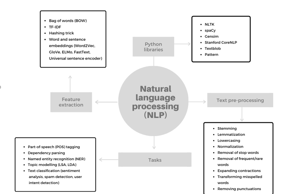
Figure 1: Natural language processing

Conclusion

We presented an introduction to the natural language processing, a multi-disciplinary field of computer science, artificial intelligence and linguistics that focuses on the interaction between computers and human language. We provided an overview of several key methods used in NLP tasks: text pre-processing, feature extraction (bag of words, TF-IDF, hashing trick) and word embeddings.

In our second article on NLP, we will continue the discussion by focusing on several advanced methodologies that often form an important of NLP solutions – part-of-speech tagging, dependency parsing, named entity recognition, topic modelling and text classification.

Natural language processing – text pre-processing, feature extraction, hashing trick and word embeddings