K-means clustering from scratch

Introduction

The amount of data produced on daily basis has steeply increased in the last decade, driven by widespread adoption of mobile devices, conversion of media and other content to digital form, the rise in number of embedded devices and many other trends.

Organizations are collecting, storing and processing these data and use it in many ways, including:

• producing business insights and identifying trends for better decision making of managers and other stakeholders,
• generating automated recommendations by using machine learning,
• improving products/services through opinion mining, anomaly detection and other techniques,
• recruiting activities.

Data scientists and others employ a wide range of approaches for analysis of their data. An important set of methods involves clustering or segmenting of data in groups of data points so that data points in the same group are very similar and at the same time distinct from data points in other groups.

Clustering belongs to the unsupervised machine learning algorithms, which means that there is no target variable to help in the learning process or in finding structures in the data.

Business uses of clustering

Clustering is widely used in many different industries and sectors. Most common business cases include:

• customer segmentation
• inventory categorization
• image segmentation
• document categorization
• call detail record (CDR) analysis
• recommendation engines
• anomaly, fraud detection

One of the most popular clustering algorithms available is the K-means algorithm, it is easy to implement and very efficient.

K-means algorithm

The K-means algorithm is an unsupervised machine learning algorithm that iteratively searches for the optimal division of data points into a pre-determined number of clusters (represented by variable K), where each data instance is a “member” of only one cluster.

K-means algorithm tries to distribute the data points in a way which makes the data points within clusters close to each other and as distant as possible from data points in other clusters.

K-means algorithm is distance-based, and its main objective is to minimize within-cluster sum of squares:

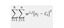
where C_i denotes centroid for cluster i, x_j data point j and w_ij is equal to 1 if point j is in cluster i and 0 otherwise.

K-means clustering belongs to the class of unsupervised learning algorithms. The main idea is to partition a group of objects in a pre-defined number of clusters in a way that objects in the same cluster are more similar to each other than to other objects from other clusters.

The algorithm to detemine the final set of clusters can be divided in the following steps:

1. choose k – the number of clusters

2. select k random points as the initial centroids

3. assign each data point to the nearest cluster based on the distance of the data point to the centroid (use Euclidean distance)

4. calculate the new coordinates of all clusters centroids by averaging coordinates over all clusters members

5. repeat steps 3. and 4. until the clusters members do not change anymore (no transitions between clusters)

Data

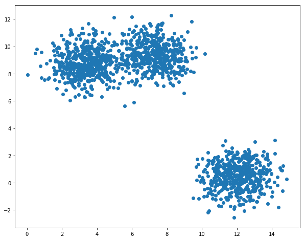
Let us first generate a set of data points from multivariate normal distribution:

import numpy as np
import matplotlib.pyplot as plt
import random 
import os

#generate population
number_of_centres=3
number_of_points_per_centre=500
np.random.seed(1)
colors = ["red", "blue" , "green", "orange"]
img_counter=0
for i in range(number_of_centres): 
    means=[15*np.random.random(),10*np.random.random()]
    a=np.random.multivariate_normal(means,[[1,0],[0,1]],number_of_points_per_centre)    
    if i==0:
        X=a
    else:    
        X=np.vstack((X,a))
plt.figure(figsize=(10,8))
plt.scatter(X[:,0],X[:,1])

We need some functions to perform main steps of the algorithm:

def recalculate_clusters(X,centroids,k):
    clusters=dict()
    for i in range(k):
        clusters[i]=[]
    for data in X:
        e_distance=[]
        for j in range(k):
            e_distance.append(np.linalg.norm(data - centroids[j]))
        clusters[e_distance.index(min(e_distance))].append(data)
    return clusters    

def recalculate_centroids(centroids,clusters,k):
    for i in range(k):
        centroids[i]=np.average(clusters[i],axis=0)
    return centroids

Iterating through the algorithm:

k=3
centroids={}
for i in range(k):
    centroids[i]=X[i]
    
for i in range(10):        
    clusters=recalculate_clusters(X,centroids,k)  
    centroids=recalculate_centroids(centroids,clusters,k)
    plot_clusters(centroids,clusters,k)

and plotting the clusters with:

def plot_clusters(centroids,clusters,k):
    plt.figure(figsize=(10,8))  
    area = (20)**2
    for i in range(k):
        for cluster in clusters[i]:
            plt.scatter(cluster[0],cluster[1],c=colors[i % 3])          
        plt.scatter(centroids[i][0],centroids[i][1],s=area,marker='^', edgecolors='white',c=colors[i % 3])

gives the following evolution to final cluster composition:

K-means algorithm drawbacks

Although K-means algorithm is relatively easy to implement and very fast, it is important to be aware of its limitations. One drawback is that the results of the K-means algorithm are sensitive to initialization of centroids and we may not achieve the globally optimal solution.

K-means algorithm also assumes that data in clusters is distributed spherically around the centre point of the cluster and may lead to suboptimal results on data sets with non-spherical clusters or on data sets with outliers.

Further, we need to provide in advance the number of clusters for the K-means algorithm, it cannot learn the value of this parameter from the data.

We will now in turn discuss these limitations of the K-means algorithm and how to address them.

Sensitivity of K-means to initialization of centroids

In our example above, we used a specific random seed (2) in randomly selecting initial centroids from among the data points. If we use a different random seed (1 instead of 2):

centroids,clusters=k_means(X,number_of_centres,1,initialize_centroids_default,100)

plot_clusters(centroids,clusters,number_of_centres,X,'K-means clustering from scratch')

our K-means clustering algorithm produces a suboptimal result:

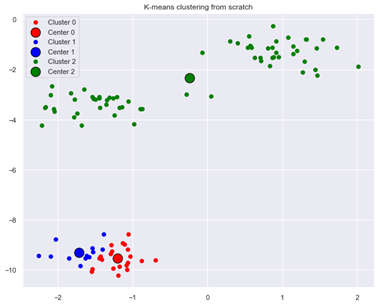
Figure 3: Suboptimal result from K-means clustering when using different initial centroids

We can resolve the problems with suboptimal initialization of centroids in several ways. One approach is to run the K-means algorithm for several different starting centroids and select the one with the lowest inertia (within-cluster sum-of-squares). Scikit-learn implementation of the K-means algorithm uses by default 10 consecutive runs with different centroid seeds.

Another approach is to use an improved method for centroid initialization. The most known algorithm for selecting initial seeds is the k-means++ algorithm.

k-means++ algorithm

k-means++ algorithm seeds the initial cluster centres by selecting the first centre from among the data points. The 2^nd and further centres are selected randomly from remaining data points, but with probability of selecting a data point being proportional to its squared distance to the nearest existing cluster centre.

k-means++ algorithm coded from scratch is as follows, using roulette wheel selection method:

def k_means_plus2(X,number_of_centres):

centroids = X[np.random.permutation(X.shape[0])[:1]]

for i_ in range(number_of_centres-1):

distances2 = []

# iterate over all points

for point_index in range(X.shape[0]):

point_vector = X[point_index]

distances2.append(min([(np.inner(point_vector-centroids[centroid_index],point_vector-centroids[centroid_index])) for centroid_index in range(len(centroids))]))


# implementing roulette wheel selection

distances2 = distances2/sum(distances2)

probs_cumsum = [sum(distances2[:i+1]) for i in range(len(distances2))]

random_between_0_1 = random.random()

for point_index in range(X.shape[0]):

if random_between_0_1 < probs_cumsum[point_index]:

n = point_index

break

centroids=np.vstack((centroids,X[n]))

return centroids

 

Applying k-means algorithm with random seed 1 and with k-means++ initialization now leads to optimal clustering:

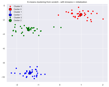
Figure 4: Optimal result from K-means clustering with k-means++ initialization

For reference, we are also adding code that uses alternative, Scikit-learn implementation of K-means algorithm:

kmeans_model = KMeans(n_clusters=3)

kmeans_model.fit(X)

y_pred = kmeans_model.predict(X)

sklearn_clusters=defaultdict(list)

classes=list(set(y_pred))

for point_index,cluster_index in enumerate(y_pred):

sklearn_clusters[cluster_index].append(point_index)

plot_clusters(kmeans_model.cluster_centers_,sklearn_clusters,number_of_centres,X,'K-means clustering with scikit-learn')

K-means algorithm on non-spherical data

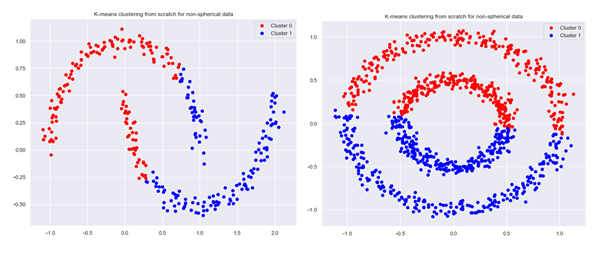
As mentioned earlier, K-means algorithm encounters difficulties when used on non-spherical data. To illustrate this, we will generate two example data sets with the help of functions make_moons and make_circles:

X, y = make_moons(300, noise=.05, random_state=0)

centroids,clusters=k_means(X,2,1,k_means_plus2,100)

plot_clusters(None,clusters,2,X,’K-means clustering from scratch for non-spherical data’)

X, y = make_circles(n_samples=1000, noise=.05, factor=.5, random_state=0)

centroids,clusters=k_means(X,2,1,k_means_plus2,100)

plot_clusters(None,clusters,2,X,’K-means clustering from scratch for non-spherical data’)

 

We can see that our K-means algorithm using k-means++ initialization leads to clustering that is different from what we would intuitively expect:

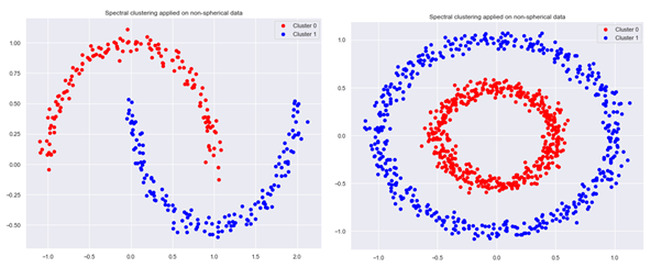
Spectral clustering

When dealing with non-spherical data or other complex structures of data points, an improved clustering can often be obtained by using the spectral clustering method instead of K-means.

Spectral clustering converts the data into a similarity graph with each vertex in the graph representing a data point. There are several methods for transforming data points with pairwise similarities or distances into a graph:

• epsilon-neighbourhood graph: we connect data points with pairwise distances lower than epsilon,
• k-nearest neighbour graph: we connect vertex x with vertex y if y is among the k-nearest neighbours of x,
• fully connected graph: each point is connected to every other point, weighted by similarity.

Next step of the spectral clustering method is determination of the graph Laplacian and calculation of its eigenvalues and eigenvectors. We then cluster the points in this transformed space by using K-means or some other traditional clustering algorithm.

Spectral clustering algorithm is implemented in Scikit-learn, we can apply it to our problem with the following code:

def spectral_clustering(X,number_of_clusters,title):

    kmeans_sc_model = SpectralClustering(n_clusters=number_of_clusters, affinity='nearest_neighbors',assign_labels='kmeans')

    kmeans_sc_model.fit(X)

    y_pred = kmeans_sc_model.fit_predict(X)


    sklearn_clusters=defaultdict(list)

    classes=list(set(y_pred))

    for point_index,cluster_index in enumerate(y_pred):

        sklearn_clusters[cluster_index].append(point_index)

    plot_clusters(None,sklearn_clusters,number_of_clusters,X,title)

obtaining an improvement in clustering for non-spherical data sets:

Optimal number of clusters – Elbow method

K-means algorithm requires only one parameter – K, the number of centroids or clusters. There are different methods available to determine the optimal value of K. One of the most common methods involves trying out different values of K, determining within-cluster sum of squares for each K and plotting the resulting relation.

The optimal number of clusters is then chosen as the point in the chart where a further increase in number of clusters will cause only a relatively small decrease in within-cluster sum of squares, while decrease in number of clusters will cause a sharp increase in the within-cluster sum of squares.

This point is known as the elbow point and visually indicates the optimal value of K for the K-means algorithm.

Another method for determining optimal number of clusters for the K-means algorithm is the Silhouette analysis.

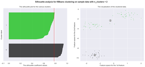
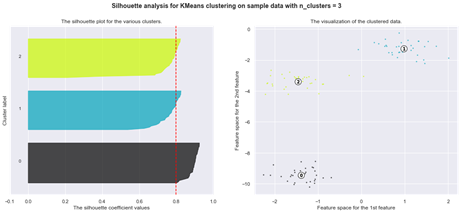
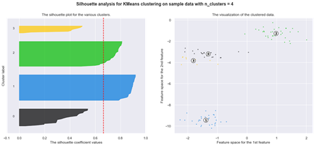
Silhouette analysis

The silhouette plot shows how close a point in one cluster is to data points in the neighbouring clusters. It allows us to visually assess the parameters like the number of clusters. This metric has a range between -1 and 1.

Using silhouette analysis on our data set produces the following silhouette scores:

Finally, let us examine another type of a clustering problem where the standard K-means algorithm may encounter difficulties and where a different method may be more appropriate: data with outliers.

Clustering of data with outliers frequently arises in the problem of anomaly detection. In this case, K-means algorithm ensures that each data point is part of one of the clusters, even though it may be an outlier.

What is required is an alternative approach and one of the possible methods to apply in such case is Density-Based Spatial Clustering of Applications with Noise or DBSCAN.

Density-Based Spatial Clustering of Applications with Noise (DBSCAN)

DBSCAN is a density-based algorithm that does not require number of clusters as parameter like K-means.

It extracts dense clusters of data points and identifies the remaining points as outliers.

DBSCAN is controlled by two parameters:

• epsilon: the radius of “neighbourhood” around data point. If distance between two points is lower than epsilon, they are treated as neighbours,
• minPts: minimum number of points within epsilon radius.

DBSCAN classifies all data points in three categories:

• data point is considered a core point if minimum minPts points are within epsilon from the point (including data point itself),
• data point x is bordered point if epsilon sized neighbourhood contains less than minPts points, but the point x is reachable from another core point x,
• all data points that are not core or bordered are considered as outliers.