Recommender systems are methods that predict users’ interests and make meaningful recommendations to them for different items, such as songs to play on Spotify, movies to watch on Netflix, news to read about your favourite newspaper website or  products to purchase on Amazon.

Recommender systems can be distinguished primarily by the type of information that they use. Content-based recommenders rely on attributes of users and/or items, whereas collaborative filtering uses information on the interaction between users and items, expressed in the so-called user-item interaction matrix.

Recommender systems are generally divided into 3 main approaches: content-based, collaborative filtering, and hybrid recommendation systems (see Fig. 1).

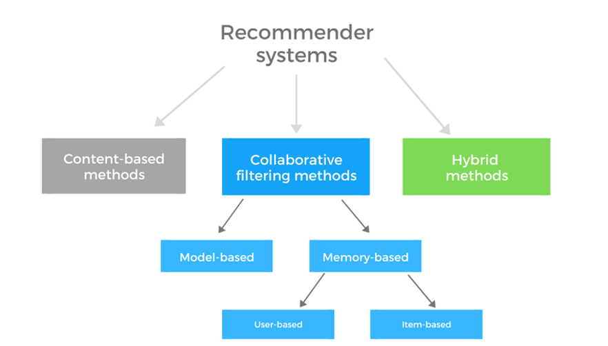
Figure 1: Types of recommender systems

What are content-based recommender systems?

Content-based recommender systems generate recommendations by relying on attributes of items and/or users. User attributes can include age, sex, job type and other personal information. Item attributes on the other hand, are descriptive information that distinguishes individual items from each other. In case of movies, this could include title, cast, description, genre and others.

By relying on features, those of users and items, content-based recommender systems are more like a traditional machine learning problem than is the case for collaborative filtering. Content-based method uses item-based or user-based features to predict an action of the user for a given item. User’s action can be a specific rating, a buy decision, like or dislike, a decision to view a movie and similar.

One of the advantages of content-based recommendation is user independence – to make recommendations to a user, it does not require information about other users, unlike collaborative filtering. This makes content-based approach easier to scale. Another benefit is that the recommendations are more transparent, as the recommender can more clearly explain recommendation in terms of the features used.

Content-based approach also has its drawbacks, one is over-specialization – if the user is only interested in specific categories, recommender will have difficulty recommending items outside of this scope, leading to user remaining in its current circle of items/interests. Content-based approaches also often require domain knowledge to produce relevant item and user features.

We will now build an implementation of content-based recommender in python, using the MovieLens dataset.

Content-based recommender system for recommendation of movies

Our recommender system will be able to recommend movies to us, based on movie plots and based on combination of features, such as top actors, director, keywords, producer and screenplay writers of the movies.

First, we load the models:

import pandas as pd

import ast

from sklearn.feature_extraction.text import CountVectorizer

from sklearn.feature_extraction.text import TfidfVectorizer

from sklearn.metrics.pairwise import cosine_similarity

import seaborn as sns

import numpy as np

import matplotlib.pyplot as plt

 

Next, we import data from https://www.kaggle.com/rounakbanik/the-movies-dataset and https://grouplens.org/datasets/movielens/latest/:

df_data = pd.read_csv(‘movies_metadata.csv’, low_memory=False)

One of the pre-processing steps for our recommender involves removing movies which have low number of votes:

df_data = df_data[df_data['vote_count'].notna()]

plt.figure(figsize=(20,5))

sns.distplot(df_data['vote_count'])

plt.title("Histogram of vote counts")

# determine the minimum number of votes that the movie must have to be included 

min_votes = np.percentile(df_data['vote_count'].values, 85)

# exclude movies that do not have minimum number of votes

df = df_data.copy(deep=True).loc[df_data['vote_count'] > min_votes]

Content-based recommender that recommends movies based on similarity of movie plots

Our first content-based recommender will have a goal of recommending movies which have a similar plot to a selected movie.

We will use “overview” feature from our dataset:

# removing rows with missing overview

df = df[df['overview'].notna()]

df.reset_index(inplace=True)


# processing of overviews

def process_text(text):

    # replace multiple spaces with one

    text = ' '.join(text.split())

    # lowercase

    text = text.lower()

    return text

df['overview'] = df.apply(lambda x: process_text(x.overview),axis=1)

To compare movie plots, we first need to compute their numerical representation. There are various approaches we can use, from bag of words, word embeddings to TF-IDF, we will select the latter.

TF-IDF approach

TF-IDF of a word in a document which is part of a larger corpus of documents is a combination of two values. One is term frequency (TF), which measures how frequently the word occurs in the document.

However, some of the words, such as “the” and “is”, occur frequently in all documents and we want to downscale the importance of such words. This is accomplished by multiplying TF with the inverse document frequency.

This ensures that only those words are considered important for the document that are frequent in this document but more rarely present in the rest of the corpus.

To build the TF-IDF representation of movie plots we will use the TfidfVectorizer from scikit-learn. We first fit TfidfVectorizer on train data set of movie plot descriptions and then transform the movie plots into TF-IDF numerical representation:

tf_idf = TfidfVectorizer(stop_words='english')

tf_idf_matrix = tf_idf.fit_transform(df['overview']);

 

Now that we have numerical vectors, representing each movie plot description, we can compute similarity of movies by calculating their pair-wise cosine similarities and storing them in cosine similarity matrix:

# calculating cosine similarity between movies

cosine_similarity_matrix = cosine_similarity(tf_idf_matrix, tf_idf_matrix)

With cosine similarity matrix computed, we can define the function “recommendations” that will return top recommendations for a given movie.

The function first determines the index of the input movie, retrieves the similarities of movies with selected movie, sorts them and returns the titles of movies with the highest similarity to the selected movie.

def index_from_title(df,title):

return df[df['original_title']==title].index.values[0]


# function that returns the title of the movie from its index

def title_from_index(df,index):

return df[df.index==index].original_title.values[0]


# generating recommendations for given title

def recommendations( original_title, df,cosine_similarity_matrix,number_of_recommendations):

index = index_from_title(df,original_title)

similarity_scores = list(enumerate(cosine_similarity_matrix[index]))

similarity_scores_sorted = sorted(similarity_scores, key=lambda x: x[1], reverse=True)

recommendations_indices = [t[0] for t in similarity_scores_sorted[1:(number_of_recommendations+1)]]

return df['original_title'].iloc[recommendations_indices]

 

We can now produce our recommendation for a given film, e.g. ‘Batman’:

recommendations(‘Batman’, df, cosine_similarity_matrix, 10)

3693    Batman Beyond: Return of the Joker    

5962    The Dark Knight Rises                 

7379    Batman vs Dracula                     

5476    Batman: Under the Red Hood            

6654    Batman: Mystery of the Batwoman       

3911    Batman Begins                         

6334    Batman: The Dark Knight Returns, Part

1770     Batman & Robin                        

4725    The Dark Knight                       

709     Batman Returns   

 

Content-based recommender based on keywords, actors, screenplay, director, producer and genres features

The recommender based on overview is of a limited quality as it considers only the movie plot.

We will now explore a different recommender, which gives more focus to other metadata (keywords, actors, director, producer, genres and screenplay authors) when recommending movies.

To use additional metadata, we first need to extract it from separate files, keywords.csv and credits.csv, and merge it with the main pandas dataframe:

df_keywords = pd.read_csv('keywords.csv')

df_credits = pd.read_csv('credits.csv')

# Some ids have irregular format, so we will remove them

df_cb = df_data.copy(deep=True)[df_data.id.apply(lambda x: x.isnumeric())]

df_cb['id'] = df_cb['id'].astype(int)

df_keywords['id'] = df_keywords['id'].astype(int)

df_credits['id'] = df_credits['id'].astype(int)

# Merging keywords, credits of movies with main data set

df_movies_data = pd.merge(df_cb, df_keywords, on='id')

df_movies_data = pd.merge(df_movies_data, df_credits, on='id')

 

Again, we will keep only the movies with highest vote counts using similar code as previously.

We next create a new feature for each movie, which consists of top 4 actors in the movie. We also concatenate and lowercase the name and surname of actors. We namely want e.g. Tom of Tom Hanks to be distinct from Tom in Tom Selleck, replacing both names with tomhanks and tomselleck, respectively:

max_number_of_actors = 4

def return_actors(cast):

actors = []

count = 0

for row in ast.literal_eval(cast) :

if count<max_number_of_actors:

actors.append(row['name'].lower().replace(" ",""))

else:

break

count+=1

return ' '.join(actors)


df_movies['actors']=df_movies.apply(lambda x: return_actors(x.cast),axis=1)

We will now create similar features for director, screenplay and producer of movies. To simplify, we only use first person detected per job type.

def return_producer_screenplay_director(crew,crew_type):

persons = []

for row in ast.literal_eval(crew) :

if row['job'].lower()==crew_type:

persons.append(row['name'].lower().replace(" ",""))

return ' '.join(persons)


df_movies['director']=df_movies.apply(lambda x: return_producer_screenplay_director(x.crew,'director'),axis=1)

df_movies['screenplay']=df_movies.apply(lambda x: return_producer_screenplay_director(x.crew,'screenplay'),axis=1)

df_movies['producer']=df_movies.apply(lambda x: return_producer_screenplay_director(x.crew,'producer'),axis=1)

After generating individual metadata, we merge them in a single feature with the ability to individually weight different features. This allows us to build highly flexible recommenders, as we will see later on.

# relative importance of different features

w_genres = 2

w_keywords = 3

w_actors = 3

w_director = 1

w_producer = 1

w_screenplay = 1

# function for merging features

def concatenate_features(df_row):

genres = []

for genre in ast.literal_eval(df_row['genres']) :

genres.append(genre['name'].lower())

genres = ' '.join(genres)

keywords = []

for keyword in ast.literal_eval(df_row['keywords']) :

keywords.append(keyword['name'])

keywords = ' '.join(keywords)

return ' '.join([genres]*w_genres)+' '+' '.join([keywords]*w_keywords)+' '+' '.join([df_row['actors']]*w_actors)+' '+' '.join([df_row['director']]*w_director)+' '+' '.join([df_row['producer']]*w_producer)+' '+' '.join([df_row['screenplay']]*w_screenplay)

 

df_movies['features'] = df_movies.apply(concatenate_features,axis=1)

# pre-processing text of features

def process_text(text):

# replace multiple spaces with one

text = ' '.join(text.split())

# lowercase

text=text.lower()

return text

df_movies['features'] = df_movies.apply(lambda x: process_text(x.features),axis=1)

 

After generating the feature, we again need to vectorize it. We will not use TF-IDF, as it reduces the importance of words which occur in many documents, in our case this e.g. also includes actors, directors, screenplay writer, producers.

We will thus use CountVectorizer for this purpose.

vect = CountVectorizer(stop_words='english')

vect_matrix = vect.fit_transform(df_movies['features'])

cosine_similarity_matrix_count_based = cosine_similarity(vect_matrix, vect_matrix)

Example recommendations:

recommendations(‘Toy Story’, df_movies, cosine_similarity_matrix_count_based, 10)

4252    Toy Story 3                5823    Toy Story That Time Forgot 785     Small Soldiers             5702    Hawaiian Vacation          1358    Toy Story 2                273     Pinocchio                  1680    The Transformers: The Movie833     Child’s Play               966     Toys                       4836    Ted     

The usage of relative weights to control importance of different metadata allows us to quickly build a new recommender focused on other aspects of movies.

We can e.g. increase weight for the director to recommend movies that are highly likely directed by the same director as the input movie:

w_director = 100

df_movies['features'] = df_movies.apply(concatenate_features,axis=1)

vect = CountVectorizer(stop_words='english')

vect_matrix = vect.fit_transform(df_movies['features'])

cosine_similarity_matrix_count_based = cosine_similarity(vect_matrix, vect_matrix)

recommendations('Toy Story', df_movies, cosine_similarity_matrix_count_based, 8)

4837    Tin Toy                

4860    Knick Knack            

3182    Luxo Jr.               

1358    Toy Story 2            

1012    A Bug’s Life           

4532    Cars 2                 

5423    Mater and the Ghostlight

3268    Cars       

A quick search shows that all of the movies recommender were directed by the director of Toy Story – John Lasseter.

Conclusion

In this article, we have introduced several content-based recommender systems in python, using MovieLens data set.

Recommender systems utilize big data about our interactions with items and try to find patterns which show what items are most popular with users that are similar to us or find items that are most similar to items that we have purchased in the past.

Besides content-based method used in this article, recommenders are also often using collaborative filtering approach or a combination of both, known as hybrid methods, which try to combine both main approaches in a way which minimizes the drawbacks of any of the individual methods. Hybrid recommenders are the most common type of recommenders, found in online platforms today.