Recommender systems are methods that try to predict users’ interests from their historical behaviour and based on that make recommendations for different items that may be of interest to them.

Netflix, with its “The Netflix Prize”, was one of the first to highlight the importance of recommender systems in modern e-commerce systems. Today’s recommender system are broadly divided into two groups, depending on the type of information they utilize to make recommendations:

– content based recommender systems,

– collaborative filtering recommender systems.

Content-based recommenders rely primarily on features of users/items to make a recommendation, whereas collaborative filtering utilizes information on interaction between users and items. These interaction can be efficiently captured in the user-interaction matrix R, where element R_ij represents the interaction of user i with item j. Interaction value can be binary (whether user i has bought item j) or of some other form (e.g. rating from 1 to 5 given by the user to the item).

In our article, we will consider collaborative filtering methods which are further subdivided into two groups: memory-based methods and model-based methods. Memory-based methods do not build a model to capture the user-item interactions, they directly use the information stored in user-item interaction matrix to produce a recommendation.

Memory-based method can be further subdivided into user-based and item-based methods. Main idea behind item-based approach is to first determine a set of items that are most similar to the test item, we will demonstrate below an example of applying an item-based approach to recommendation of movies. More often found in modern recommenders are however model-based methods, either as standalone implementations or (more often) as part of hybrid recommenders.

Funk matrix factorization method

Model-based methods assume that a lower dimensional, latent model can explain the observed user-item interactions.

One approach to determining these models this was popularized as part of the Netflix prize competition – Matrix Factorization (MF).

During competition, Simon Funk (https://sifter.org/simon/journal/20061211.html) explored the idea that the user’s rating of a movie A can be structured as the sum of preferences of this user about the various aspects of the movie A. Aspect of a movie e.g. be its genre.

The prediction for the rating of a movie is then a vector product:

where represents the values of the aspects/features of the movie m and represents the weight that the user u gives to each aspect/feature. Note that although the MF Funk approach is sometimes referred to as SVD approach, it does not actually use Singular value decomposition.

The MF Funk approach reduces the user-interaction matrix (usually large and sparse) into a product of two matrices that are much smaller, and which represent user and item representations. In our article, we will implement an improvement of the matrix factorization approach – SVD++ method.

Implementing item-based collaborative filtering

Loading the libraries:

import pandas as pd

import ast

from sklearn.metrics.pairwise import cosine_similarity

import seaborn as sns

import numpy as np

import matplotlib.pyplot as plt

from sklearn.neighbors import NearestNeighbors

from scipy.sparse import csr_matrix

from surprise import Reader, Dataset

from surprise.model_selection import train_test_split

from surprise import SVDpp, accuracy

from surprise.model_selection import cross_validate

from collections import defaultdict

from surprise import SVD, SVDpp, NMF

from surprise import SlopeOne, CoClustering

import matplotlib

Loading MovieLens data from https://www.kaggle.com/rounakbanik/the-movies-dataset and https://grouplens.org/datasets/movielens/latest/.

df_movies = pd.read_csv('movies.csv')

df_ratings = pd.read_csv('ratings.csv')

Exploratory data analysis:

ratings_count = df_ratings['rating'].value_counts().sort_index(ascending=True)

plt.figure(figsize=(12,8))

ax = ratings_count.plot.bar()

ax.set_xlabel("Rating")

ax.set_ylabel("Number of votes");

ax.set_title("Distribution of votes by rating");

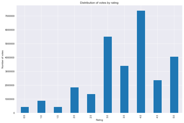
Figure 1: distribution of movie votes by rating

We can see that most of the ratings for movies are equal or larger than 3.

Most movies do not have a large number of ratings:

df = df_ratings[['movieId','userId']].groupby(['movieId']).agg(['count']).sort_values(('userId','count'),ascending=False)

plt.figure(figsize=(15,8))

sns.set_style("darkgrid")

sns.lineplot(data=df[('userId', 'count')].values)

plt.title("Rating frequency of movies")

plt.xlabel("Movie id")

plt.ylabel("Number of ratings");

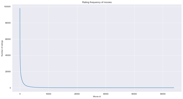
Figure 2: Rating frequency of movies

min_ratings = 500

print("Number of movies which have more than {} ratings: {}".format(min_ratings, len(df[df[('userId', 'count')]>=min_ratings])))

Number of movies which have more than 500 ratings: 5550. We will exclude rarely rated movies to make our recommendation engine more relevant:

df_top_movies = df[df[('userId', 'count')]>=min_ratings]

df_ratings_with_top_movies = df_ratings[df_ratings['movieId'].isin(list(df_top_movies.index))]

To make recommender more relevant, we will also exclude users that did not rate at least 200 movies.

min_movies_rated = 200

df_users = df_ratings_with_top_movies[['movieId','userId']].groupby(['userId']).agg(['count']).sort_values(('movieId','count'),ascending=False)

df_top_rating_users = df_users[df_users[('movieId', 'count')]>=min_movies_rated]

top_rating_users = list(df_top_rating_users.index)

df_final=df_ratings_with_top_movies[df_ratings_with_top_movies['userId'].isin(top_rating_users)]

Item-based collaborative filtering

In item-based collaborative filtering approach, all items are sorted according to their similarity to the selected item. Similarity measure can be cosine of the angle between the rows of corresponding item in the item-user matrix.

Let us first use pivoting to build the item-user matrix, with movies in rows and users in columns. We will fill missing values with 0.

df_user_item_matrix = df_final.pivot(index='movieId',columns='userId',values='rating').fillna(0)

As most of the values in our matrix are 0, we will employ sparse matrix representation:

user_item_matrix_sparse = csr_matrix(df_user_item_matrix.values)

Next, we build and train the knn nearest neighbors model:

model = NearestNeighbors(n_neighbors=30, metric='cosine', algorithm='brute', n_jobs=-1)

model.fit(user_item_matrix_sparse)

Finally, we build a recommender function and use it to return movie recommendations for given test movie:

index_to_movie = dict()

df_titles_movies = df_movies.set_index('movieId').loc[df_user_item_matrix.index]

count = 0

for index, row in df_titles_movies.iterrows():

    index_to_movie[count]=row['title']

    count +=1


def recommender(model, user_item_matrix_sparse, df_movies, number_of_recommendations, movie_index):

    main_title = index_to_movie[movie_index]

    dist, ind = model.kneighbors(user_item_matrix_sparse[movie_index], n_neighbors=number_of_recommendations+1)

    dist = dist[0].tolist()

    ind = ind[0].tolist()

    titles = []

    for index in ind:

        titles.append(index_to_movie[index])

    recommendations = list(zip(titles,dist))    

    # sort recommendations

    recommendations_sorted = sorted(recommendations, key = lambda x:x[1])

    # reverse recommendations, leaving out the first element 

    recommendations_sorted.reverse()

    recommendations_sorted = recommendations_sorted[:-1]

    print("Recommendations for movie {}: ".format(main_title))

    count = 0

    for (title, distance) in recommendations_sorted:

        count += 1

        print('{}. {}, recommendation score = {}'.format(count, title, round(distance,3)))

recommender(model, user_item_matrix_sparse, df_movies, 10, 1)

Recommendations for movie Jumanji (1995):

Toy Story (1995), recommendation score = 0.39
Aladdin (1992), recommendation score = 0.39
Mrs. Doubtfire (1993), recommendation score = 0.388
Forrest Gump (1994), recommendation score = 0.385
Independence Day (a.k.a. ID4) (1996), recommendation score = 0.38
Men in Black (a.k.a. MIB) (1997), recommendation score = 0.379
Home Alone (1990), recommendation score = 0.378
Mask, The (1994), recommendation score = 0.367
Lion King, The (1994), recommendation score = 0.362
Jurassic Park (1993), recommendation score = 0.358

Model-based model of collaborative filtering with SVD++, using surprise library

In the second part of our notebook, we will consider another type of collaborative filtering – model-based approach. Instead of memory based approach, we will try to apply SVD++ approach. SVD++ is an improvement on the Matrix-factorization approach used by Simon Funk in the Neflix challenge.

Matrix-factorization approach factorizes the user-item matrix as the product of two matrices, with rows in the first matrix representing latent factors for a user and the columns in the second matrix representing features of each item. To avoid overfitting, one also often employs regularization, especially when using a large number of latent factors.

SVD++ approach improves on Matrix-factorization approach by including not only explicit ratings, but also implicit ones (e.g. purchases, likes, etc.). Another difference is that SVD++ adds user and item bias terms to the term for MF as defined in Simon Funk approach.

Suppose that we have a user Y that is biased and gives 0.2 lower ratings than the average and that movie A is worser than the average movie, receiving 0.3 lower rating on average. This bias correction would then be -0.2-0.3=-0.5.

We will use SVD++, as implemented in the popular python library for building recommender systems – surprise (https://github.com/NicolasHug/Surprise).

To speed up calculations, we will only consider a smaller subset of the original data set, prepared in the first part of our notebook.

df_SVD = df_final.sample(frac=0.01, random_state=10).reset_index(drop=True)

By default, surprise library assumes ratings to be in range 1 to 5. We will thus pass minimum and maximum ratings of our data set.

minimum_rating = min(df_SVD['rating'].values)

maximum_rating = max(df_SVD['rating'].values)

print("Minimum/maximum ratings: {}/{} ".format(minimum_rating,maximum_rating))

Minimum/maximum ratings: 0.5/5.0

Next, we load our dataset to surprise by using its Reader class.

reader = Reader(rating_scale=(minimum_rating,maximum_rating))

data = Dataset.load_from_df(df_SVD[['userId', 'movieId', 'rating']], reader)

As mentioned before, we will use SVD++ for our algorithm.

algo = SVDpp()

algo.fit(data.build_full_trainset());

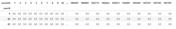
As expected, most of the elements of user-item matrix are 0. Let us select user with userId=4 and try to predict its rating for movie with movieId=10. When passing ids to surprise methods it is important to be aware that surprise package operates with raw ids and inner ids. Raw ids are ids as defined in the ratings files or in respective pandas dataframes.

Predict method is one of the methods that use and return raw ids, it is important however to pass the ids as strings:

user_id = '4'

movie_id = '10'

prediction = algo.predict(uid=user_id, iid=movie_id)

print("Predicted rating of user with id {} for movie with id {}: {}".format(user_id, movie_id, round(prediction.est,3)))

Predicted rating of user with id 4 for movie with id 10: 3.455

Next, we will build a function that will return recommendations, chosen from movies that the user has not rated yet.

def recommendations_from_SVDpp(user_id, df_user_item_matrix_SVD, algo, n_recommendations): 

    # determine list of unrated movies by user_id

    list_of_unrated_movies = np.nonzero(df_user_item_matrix_SVD.loc[user_id].to_numpy() == 0)[0]

    # set up user set with unrated movies

    user_set = [[user_id, item_id, 0] for item_id in list_of_unrated_movies]


    # generate predictions

    predictions = algo.test(user_set)


    top_n_recommendations = defaultdict(list)

    for user_id, item_id, _, est, _ in predictions:

        top_n_recommendations[user_id].append((item_id, est))


    for user_id, ratings in top_n_recommendations.items():

        ratings.sort(key=lambda x: x[1], reverse=True)

        top_n_recommendations[user_id] = ratings[:n_recommendations]


    count = 0

    print("Recommendations for user with id {}: ".format(user_id))

    for movie_index, score in top_n_recommendations[user_id]: 

        count +=1

        print('{}. {}, predicted rating = {}'.format(count, df_movies[df_movies['movieId']==movie_index]['title'].iloc[0], round(score,3)))

recommendations_from_SVDpp(4, df_user_item_matrix_SVD, algo, 10)

Recommendations for user with id 4:

Casablanca (1942), predicted rating = 4.517
Reservoir Dogs (1992), predicted rating = 4.375
Shawshank Redemption, The (1994), predicted rating = 4.354
American Beauty (1999), predicted rating = 4.354
Blade Runner (1982), predicted rating = 4.351
Godfather, The (1972), predicted rating = 4.347
My Life as a Dog (Mitt liv som hund) (1985), predicted rating = 4.275
Sunset Blvd. (a.k.a. Sunset Boulevard) (1950), predicted rating = 4.272
Wallace & Gromit: The Best of Aardman Animation (1996), predicted rating = 4.272
Raging Bull (1980), predicted rating = 4.268
City Lights (1931), predicted rating = 4.267
Third Man, The (1949), predicted rating = 4.267
Twelve Monkeys (a.k.a. 12 Monkeys) (1995), predicted rating = 4.263
Pulp Fiction (1994), predicted rating = 4.258
Dr. Strangelove or: How I Learned to Stop Worrying and Love the Bomb (1964), predicted rating = 4.232
Princess Bride, The (1987), predicted rating = 4.23
Chinatown (1974), predicted rating = 4.228
Goodfellas (1990), predicted rating = 4.207
Rear Window (1954), predicted rating = 4.19
Young Frankenstein (1974), predicted rating = 4.185

Comparison of different algorithms – SVD, SVD++, NMF, SlopeOne and Co-Clustering

Surprise library has implementations of several different based algorithms:

the k-NN inspired algorithms,
MF algorithm from Simon Funk,
SVD++ algorithm, an improvement on MF approach of Funk, taking into account implicit rating,
NMF or Non-negative Matrix Factorization,
SlopeOne algorithm,
collaborative filtering algorithm based on co-clustering.

We have implemented k-NN algorithms in first part of our notebook and already discussed MF Funk and SVD++ approaches.

Non-negative Matrix Factorization (NMF) method

NMF is an approach developed by Paatero and Tapper, whereby a matrix is factorized into two low-rank matrices: V = WxH , where all three matrices have no negative elements. In context of text mining, V can represent the matrix with documents in columns and words in rows. Columns in W can then be interpreted as topics and columns in H represent values of document with respect to given topics. By combining both, we can reconstruct the mix of words in the document from the distribution of topics and their words. More information on NMF is available at papers.nips.cc/paper/1861-algorithms-for-non-negative-matrix-factorization.pdf.

SlopeOne algorithm was introduced by Daniel Lemire and Anna Maclachlan in a paper from 2005: https://arxiv.org/abs/cs/0702144. It is relatively easy to code, while the accuracy is often comparable to some of the more complicated collaborative filtering algorithms.

Let us evaluate the performance of a selection of these different algorithms on our data set:

svd = cross_validate(SVD(), data, cv=5, n_jobs=-1, verbose=False)

svdpp = cross_validate(SVDpp(), data, cv=5, n_jobs=-1, verbose=False)

nmf = cross_validate(NMF(), data, cv=5, n_jobs=-1, verbose=False)

slope = cross_validate(SlopeOne(), data, cv=5, n_jobs=-1, verbose=False)


df_results = pd.DataFrame(columns=['Method', 'RMSE', 'MAE'])

df_results.loc[len(df_results)]=['SVD', round(svd['test_rmse'].mean(),5),round(svd['test_mae'].mean(),5)]

df_results.loc[len(df_results)]=['SVD++', round(svdpp['test_rmse'].mean(),5),round(svdpp['test_mae'].mean(),5)]

df_results.loc[len(df_results)]=['NMF', round(nmf['test_rmse'].mean(),5),round(nmf['test_mae'].mean(),5)]

df_results.loc[len(df_results)]=['SlopeOne', round(slope['test_rmse'].mean(),5),round(slope['test_mae'].mean(),5)]

display(df_results)


ax = df_results[['RMSE','MAE']].plot(kind='bar', figsize=(15,8))

ax.set_xticklabels(df_results['Method'].values)

ax.set_title('RMSE and MAE of different collaborative filtering algorithms')

plt.xticks(rotation=45)

matplotlib.rcParams.update({'font.size': 14})

plt.show();

SVD++ achieves the best performance, followed by SVD, NMF and SlopeOne.

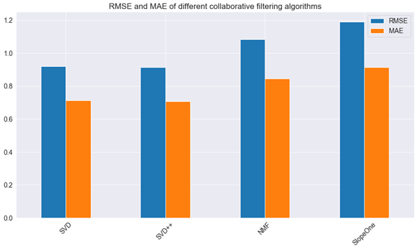
Figure 3: RMSE and MAE of different collaborative filtering algorithms

Get in Touch

Do you need consultation or have a project in mind? We would love to hear from you!

Get in Touch

Collaborative filtering Recommender System with Python – from scratch, using SVD++, item-based, model-based approaches

Funk matrix factorization method

Implementing item-based collaborative filtering

Item-based collaborative filtering

Model-based model of collaborative filtering with SVD++, using surprise library

Comparison of different algorithms – SVD, SVD++, NMF, SlopeOne and Co-Clustering

Non-negative Matrix Factorization (NMF) method

Get in Touch

Previous Post Artificial intelligence , machine learning and deep learning - AI, ML and DL

Our Blog

Next Post Best deep learning books in 2020